License: CC-BY-NC-SA 4.0
Author: Murilo M. Marinho (murilo
I found an issue
Thank you! Please report it at https://
Latex Macros
\providecommand{\myvec}[1]{{\mathbf{\boldsymbol{{#1}}}}}
\providecommand{\mymatrix}[1]{{\mathbf{\boldsymbol{{#1}}}}}
Package installation
%%capture
%pip install numpy matplotlib
%pip install numpy matplotlib --break-system-packages
Imports
%matplotlib inline
import numpy as np
import matplotlib.pyplot as plt
from math import pi, sin, cos
Definition(s)
The function(s) defined below are valid for all solutions.
def damped_pseudo_inverse(A: np.array, damping: float = 0.01):
    """Calculates the damped pseudo inverse of A"""
    if damping == 0:
        raise Exception(f"Damping is {damping} but should be different from zero")

    return A.T @ np.linalg.inv(A @ A.T + (damping ** 2) * np.eye(A.shape[0]))
PP Robot
Suppose that we have a PP robot defined by the following transformations:
a translation of along the axis of the base frame.
a rotation of 90 degrees with respect to the current frame.
a translation of along the axis of the current frame.
For FKM and Jacobian calculation, see lesson 4.
For the control parameters, see lesson 5.
def get_error(x, xd):
return x - xd
def planar_robot_pp_fkm(q: np.array) -> np.array:
q_0 = q[0]
q_1 = q[1]
return np.array([q_0,
q_1,
pi/2.0])
def planar_robot_pp_jacobian(q):
# We can leave the parameter `q` for compatibility, but it's not used for this robot.
return np.array(
[[1, 0],
[0, 1],
[0, 0]]
)
eta = 1 # Control gain
T = 0.001 # Sampling time
# A desired task-space value
xd = np.array([2.0,
2.0,
pi/10])
print(f"xd = {xd}")
# Lists to store the value of each control iteration
x_tilde_norm_list = []
t_list = []
u_norm_list = []
# Starting conditions
t = 0
q_0 = 0.0
q_1 = 0.0
q = np.array([q_0,
q_1])
# Control for 10 seconds
while t < 10:
x = planar_robot_pp_fkm(q)
x_tilde = get_error(x, xd)
J = planar_robot_pp_jacobian(q)
J_inv = damped_pseudo_inverse(J)
u = -eta * J_inv @ x_tilde
## Store values
x_tilde_norm_list.append(np.linalg.norm(x_tilde))
t_list.append(t)
u_norm_list.append(np.linalg.norm(u))
## Variable updated for the next loop
q = q + u * T
t = t + T
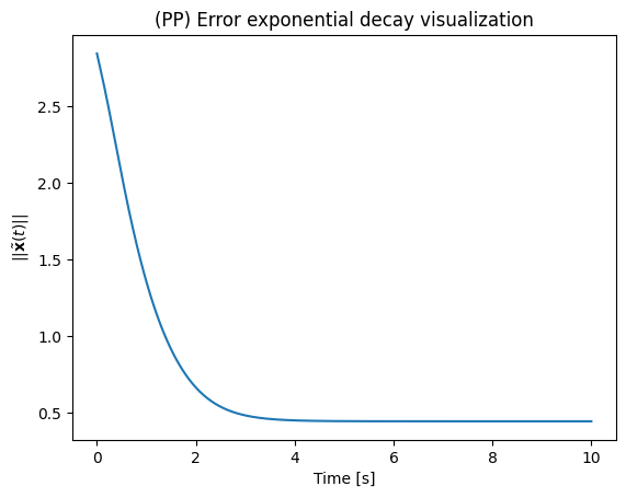
plt.plot(t_list,x_tilde_norm_list, label=f"$\\eta$={eta}")
plt.title('(PP) Error exponential decay visualization')
plt.xlabel("Time [s]")
plt.ylabel("$||\\tilde{ \\bf{x} } (t) ||$")
plt.show()xd = [2. 2. 0.31415927]
RP Robot
Suppose that we have a RP robot defined by the following transformations:
a rotation of of the base frame.
a translation of along the axis of the current frame.
For FKM and Jacobian calculation process, see lesson 4.
For the control parameters, see lesson 5.
def get_error(x, xd):
return x - xd
def planar_robot_rp_fkm(q: np.array) -> np.array:
q_0 = q[0]
q_1 = q[1]
return np.array([q_1*cos(q_0),
q_1*sin(q_0),
q_0])
def planar_robot_rp_jacobian(q):
q_0 = q[0]
q_1 = q[1]
return np.array(
[[-q_1*sin(q_0), cos(q_0)],
[ q_1*cos(q_0), sin(q_0)],
[ 1, 0]]
)
eta = 1 # Control gain
T = 0.001 # Sampling time
# A desired task-space value
xd = np.array([2.0,
2.0,
pi/10])
print(f"xd = {xd}")
# Lists to store the value of each control iteration
x_tilde_norm_list = []
t_list = []
u_norm_list = []
# Starting conditions
t = 0
q_0 = 0.0
q_1 = 0.0
q = np.array([q_0,
q_1])
# Control for 10 seconds
while t < 10:
x = planar_robot_rp_fkm(q)
x_tilde = get_error(x, xd)
J = planar_robot_rp_jacobian(q)
J_inv = damped_pseudo_inverse(J)
u = -eta * J_inv @ x_tilde
## Store values
x_tilde_norm_list.append(np.linalg.norm(x_tilde))
t_list.append(t)
u_norm_list.append(np.linalg.norm(u))
## Variable updated for the next loop
q = q + u * T
t = t + T
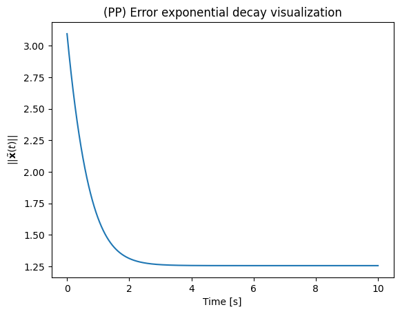
plt.plot(t_list,x_tilde_norm_list, label=f"$\\eta$={eta}")
plt.title('(PP) Error exponential decay visualization')
plt.xlabel("Time [s]")
plt.ylabel("$||\\tilde{ \\bf{x} } (t) ||$")
plt.show()xd = [2. 2. 0.31415927]