L4 Differential Kinematics

License: CC-BY-NC-SA 4.0

Author: Murilo M. Marinho (murilo.marinho@manchester.ac.uk)

Pre-requisites for the learner¶

The user of this notebook is expected to have prior knowledge in

All the content and pre-requisites of lessons 1, 2, and 3.

I found an issue¶

Thank you! Please report it at https://github.com/MarinhoLab/OpenExecutableBooksRobotics/issues

Latex Macros¶

$\providecommand{\myvec}[1]{{\mathbf{\boldsymbol{{#1}}}}}$ $\providecommand{\mymatrix}[1]{{\mathbf{\boldsymbol{{#1}}}}}$

\providecommand{\myvec}[1]{{\mathbf{\boldsymbol{{#1}}}}}
\providecommand{\mymatrix}[1]{{\mathbf{\boldsymbol{{#1}}}}}

Package installation¶

%%capture
%pip install numpy
%pip install numpy --break-system-packages

Imports¶

import numpy as np
from math import pi, sin, cos

Differential Kinematics Model (DFKM)¶

As we have seen in the previous lesson, the FKM relates configuration-space position with task-space position. For a manipulator, inserting a valid set of joint configurations into the FKM leads to the task-space values of the end-effector.

We also managed to systematise the process to find the FKM, using DH parameters. That way, the FKM of any serial-link manipulator with any number of degrees-of-freedom can be defined with a table. From the table we can derive the analytical FKM and compute it efficiently.

Although the FKM is, then, straightforward to compute, the inverse FKM does not have a general closed form for manipulators with any number of degrees-of-freedom. Naturally, there are ways to invert the FKM iteratively using its first-order derivative. This is where the differential kinematics model (DFKM) comes into play.

The DFKM is the process of finding Jacobians, because the FKM is a vector-valued function. It was once said that

"Robotics is the art of finding Jacobians."
Bruno Siciliano @ Rosenbrock Lecture Series 2024

The importance of Jacobians for robotics cannot be overstated. In conclusion, the DFKM is a central process of robotics.

Despite all the fancy words, it’s a rather simple process for simple manipulators. Let’s start with our usual toy example.

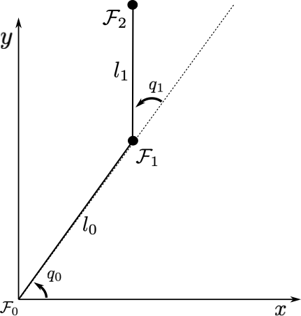
For the 2-DoF planar robot shown in the figure, let us use the FKM obtained in the previous lesson. It is given as

\mymatrix{H}^{0}_{2}( q_0, l_{0},q_1,l_{1}) \in SE(2).

(1)

Also remember that the configuration space of this manipulator is

\myvec{q} = \left[\begin{array}{c} q_0 \\ q_1 \end{array}\right].

(2)

The DFKM is the process of calculating a Jacobian relevant for a given task. Therefore, herein we obtain the Jacobian $\mymatrix{J}\left(\myvec{q}\right)$ such that

\dot{\myvec{x}}=\mymatrix{J}\left(\myvec{q}\right) \dot{\myvec{q}}

(3)

where

\myvec{x} = \left[\begin{array}{c} p_{x} \\ p_{y} \\ \phi \end{array}\right],

(4)

in which $p_{x}$ , $p_{y}$ , and $\phi$ are, respectively, the $x$ -axis position, the $y$ -axis position, and the rotation angle of $\mathcal{F}_{2}$ . Notice that $\dot{l}_{0}=\dot{l}_{1}=0$ , because, as we defined in the previous lesson, they do not vary in time.

As defined above, the Jacobian $\mymatrix{J}\left(\myvec{q}\right)$ is a function of the configuration-space values. Therefore, when computing it, we need to know at what $\myvec{q}$ .

As a second part of this toy example, let us calculate what is the end-effector velocity given a configuration-space velocity. Mathematically, let us calculate $\dot{\myvec{x}}$ when

\dot{\myvec{q}} = \left[\begin{array}{c} 5 \\ 10 \end{array}\right].

(5)

Step 1: Calculate the forward kinematics by hand¶

It is not possible to calculate the Jacobian without the FKM.

We saw how to do that in the previous lesson, so here is the answer for this robot.

\mymatrix{H}^{0}_{2} = \left[\begin{array}{ccc} \cos{(q_0 + q_1)} & -\sin{(q_0 + q_1)} & l_{0}\cos{q_0} + l_{1}\cos{(q_0 + q_1)}\\ \sin{(q_0 + q_1)} & \cos{(q_0 + q_1)} & l_{0}\sin{q_0} + l_{1}\sin{(q_0 + q_1)}\\ 0 & 0 & 1 \end{array}\right].

(6)

This means that, from inspection,

\begin{align} p_{x}&=l_{0}\cos{q_0} + l_{1}\cos{(q_0 + q_1)} \\ p_{y}&=l_{0}\sin{q_0} + l_{1}\sin{(q_0 + q_1)} \\ \phi&=q_0 + q_1 .\\ \end{align}

(7)

Step 2: Calculate the differential kinematics by hand¶

We first calculate the Jacobian by hand, because programmatically there’s nothing for us to do yet.

The analytical Jacobian is given by

\mymatrix{J} = \left[\begin{array}{ccc} \frac{\partial p_{x}}{\partial q_0} & \frac{\partial p_{x}}{\partial q_1} \\ \frac{\partial p_{y}}{\partial q_0} & \frac{\partial p_{y}}{\partial q_1} \\ \frac{\partial \phi}{\partial q_0} & \frac{\partial \phi}{\partial q_1} \end{array}\right].

(8)

As we did in class, we find each element by calculating the partial derivative of the respective task-space value with respect to the configuration-space value

\begin{align} \frac{\partial p_{x}}{\partial q_0} &= -l_{0}\sin{q_0} - l_{1}\sin{(q_0 + q_1)} \\ \frac{\partial p_{x}}{\partial q_1} &= -l_{1}\sin{(q_0 + q_1)} \\ \frac{\partial p_{y}}{\partial q_0} &= l_{0}\cos{q_0} + l_{1}\cos{(q_0 + q_1)} \\ \frac{\partial p_{y}}{\partial q_1} &= l_{1}\cos{(q_0 + q_1)} \\ \frac{\partial \phi}{\partial q_0} &= 1 \\ \frac{\partial \phi}{\partial q_1} &= 1 \end{align}

(9)

resulting in

\mymatrix{J} = \left[\begin{array}{ccc} -l_{0}\sin{q_0} - l_{1}\sin{(q_0 + q_1)} & -l_{1}\sin{(q_0 + q_1)} \\ l_{0}\cos{q_0} + l_{1}\cos{(q_0 + q_1)} & l_{1}\cos{(q_0 + q_1)} \\ 1 & 1 \end{array}\right].

(10)

Step 3: Computing the Jacobian¶

We’re now equipped to solve the first question by doing the following

# Sample values, the particular values do not matter
q_0 = pi / 4
q_1 = pi / 3
l_0 = 0.2
l_1 = 0.1

# To possibly make it easier for you to read
J_1_1 = -l_0 * sin(q_0) - l_1 * sin(q_0 + q_1)
J_1_2 = -l_1 * sin(q_0  + q_1)
J_2_1 =  l_0 * cos(q_0) + l_1 * cos(q_0 + q_1)
J_2_2 =  l_1 * cos(q_0 +  q_1)
J_3_1 = 1
J_3_2 = 1

J = np.array(
        [[J_1_1, J_1_2],
         [J_2_1, J_2_2],
         [J_3_1, J_3_2]]
)

print(f"The analytical Jacobian at {q_0} and {q_1} is {J}")

The analytical Jacobian at 0.7853981633974483 and 1.0471975511965976 is [[-0.23801394 -0.09659258]
 [ 0.11553945 -0.0258819 ]
 [ 1.          1.        ]]

With the correct definition of the Jacobian as above, we can calculate the second question as

q_dot = np.array(
        [[5],
         [10]]
)

x_dot = J @ q_dot

print(f"In these conditions, x_dot = {x_dot}")

In these conditions, x_dot = [[-2.15599552]
 [ 0.31887821]
 [15.        ]]

Suggested exercises¶

What about if the robot had 3 degrees-of-freedom, that is RRR?
What if the robot has one or more prismatic joints?
Challenge. What about if the robot had $n$ revolute degrees-of-freedom? Would it be much more complicated to solve?