%%capture
'''
(C) Copyright 2020-2025 Murilo Marques Marinho (murilomarinho@ieee.org)

     This file is licensed in the terms of the
     Attribution-NonCommercial-ShareAlike 4.0 International (CC BY-NC-SA 4.0)
     license.

 Derivative work of:
 https://github.com/dqrobotics/learning-dqrobotics-in-matlab/tree/master/robotic_manipulators
 Contributors to this file:
     Murilo Marques Marinho (murilomarinho@ieee.org)
'''

DQ7 Robot Control Basics using DQ Robotics - Part 3¶

I found an issue¶

Thank you! Please report it at https://github.com/MarinhoLab/OpenExecutableBooksRobotics/issues

Introduction¶

In the last lesson, you learned how model robotic manipulators parameterized using the DH parameters. You also learned how to use a basic controller based on the pseudo-inverse of the task Jacobian.

That was an introductory exposition to robot control, and this lesson will introduce you to the concept of task-space singularities and a particular way to address them.

%%capture
%pip install dqrobotics dqrobotics-pyplot
%pip install dqrobotics dqrobotics-pyplot --break-system-packages

from math import pi

import numpy as np

from dqrobotics import *
from dqrobotics.robot_control import DQ_PseudoinverseController, ControlObjective
from dqrobotics_extensions.pyplot import plot

import matplotlib.pyplot as plt
plt.rcParams["animation.html"] = "jshtml" # Need to output animation's videos
import matplotlib.animation as anm
from functools import partial # Need to call functions correctly for matplotlib animations

Notation¶

Keep these in mind (we will also use this notation when writting papers to conferences and journals):

$h\in \mathbb{H}$ : a quaternion. (Bold-face, lowercase character)
$\underline{h} \in \mathcal{H}$ : a dual quaternion. (Bold-face, underlined, lowercase character)
$p,t,\cdots \in {\mathbb{H}}_p$ : pure quaternions. They represent points, positions, and translations. They are quaternions for which $\textrm{Re}\left(h\right)=0$ .
$r\in {\mathbb{S}}^3$ : unit quaternions. They represent orientations and rotations. They are quaternions for which $||h||=1$ .
$\underline{x} \in$ $\underline{\mathcal{S}}$ : unit dual quaternions. They represent poses and pose transformations. They are dual quaternions for which $||h||=1$ .
$\underline{l} \in {\mathcal{H}}_p \cap$ $\underline{{\mathcal{S}}}$ : a Plücker line.
$\underline{{{\pi }}} \in \left\lbrace P\left(\underline{{{\pi }}} \right)\in {\mathbb{H}}_p \right\rbrace \cap \underline{{\mathcal{S}}}$ : a plane.
$\theta ,a,b,\cdots \in \mathbb{R}$ : real numbers.
${{q,\cdots }}\in {\mathbb{R}}^n :$ real vectors.
$J,A,B,\cdots \in {\mathbb{R}}^{m\times n} :$ real matrices.

Robot definition¶

The concepts of this lesson apply to any manipulator robot. However, to have a more concrete understanding using DQ Robotics, consider the following robot that will be used in all examples in this lesson.

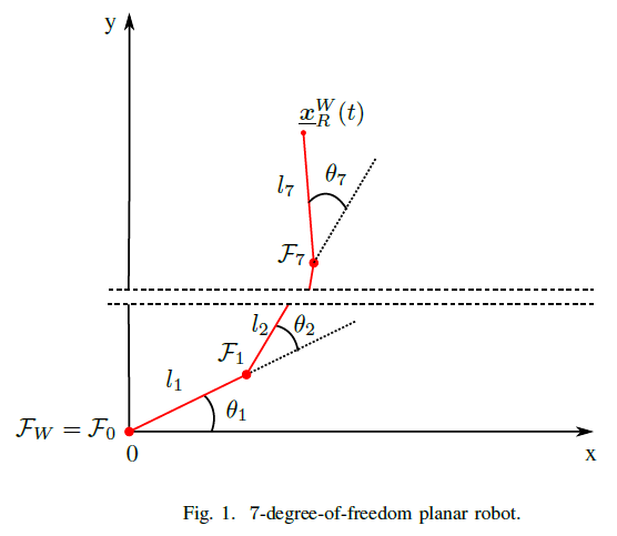
Let the robot $R$ be a 7-DoF planar robot, as drawn in Fig.1.
Let ${\mathcal{F}}_W$ be the world-reference frame.
Let ${\underline{x} }_R^W (t)\triangleq {\underline{x} }_R$ $\in$ $\underline{\mathcal{S}}$ represent the pose of the end effector.
Let $R$ be composed of seven rotational joints that rotate about their z-axis, composed in the joint-space vector $q\left(t\right)\triangleq q={\left\lbrack \theta_1 ~\theta_2 ~\theta_3 ~\theta_4 ~\theta_5 ~\theta_6 ~\theta_7 \right\rbrack }^T$ with $\theta_i \left(t\right)\triangleq \theta_i \in \mathbb{R}$ for $i=1,2,\ldots,7$ . The rotation of the reference frames of each joint coincide with the rotation of ${\mathcal{F}}_W$ when $\theta_i =0$ . The length of the joints are $l_i \in$ ${\mathbb{R}}^+ -\lbrace 0\rbrace$ .
Consider that we can freely control the joint vector $q$ .

This robot can be modeled by the following class.

from seven_dof_planar_robot_dh import SevenDofPlanarRobotDH
help(SevenDofPlanarRobotDH.kinematics)

Help on function kinematics in module seven_dof_planar_robot_dh:

kinematics()
    Returns the kinematics of the SevenDoFPlanarRobot as DQ_SerialManipulatorDH.

Let us instantiate our robot as follows

seven_dof_planar_robot = SevenDofPlanarRobotDH.kinematics()

Robot controller¶

The concepts of this lesson also apply for any of the task-space control types mentioned in the last lesson (and others). For us to have a concrete example for this lesson, let us define a translation controller based on the pseudo-inverse of the Jacobian with no damping.

translation_controller = DQ_PseudoinverseController(seven_dof_planar_robot)
translation_controller.set_control_objective(ControlObjective.Translation)
translation_controller.set_gain(10)
translation_controller.set_damping(0)

Task-space singularities¶

One important concept when controlling a robot using its task Jacobian is the concept of task-space singularities. The task-space singularities are closely related to the linear-algebra concept of singular matrices. Let us remember a few linear-algebra concepts.

Matrix rank and singularities¶

Take as an example the $3\times 3$ identity matrix

I_{3\times 3} =\left\lbrack \begin{array}{ccc} 1 & 0 & 0\\ 0 & 1 & 0\\ 0 & 0 & 1 \end{array}\right\rbrack .

(1)

I3_3 = np.eye(3)

It obviously has rank three, that is, its three rows are linearly independent.

np.linalg.matrix_rank(I3_3)

np.int64(3)

However, the following the matrix

A=\left\lbrack \begin{array}{ccc} 0 & 0 & 1\\ 0 & 0 & 1\\ 0 & 1 & 0 \end{array}\right\rbrack ,

(2)

A = np.array([[0, 0, 1],
              [0, 0, 1],
              [0, 1, 0]])

has rank two given that its first and second row are linearly dependent.

np.linalg.matrix_rank(A)

np.int64(2)

A square matrix is considered singular whenever its rank is lower than its number of rows (or columns). This means that the matrix does not have an inverse.

Moreover, non-square matrices also do not have an inverse.

Is there a way to “invert” rectangular matrices and singular matrices?

A quick review on the SVD-based inverse for full-rank matrices¶

Suppose that we want to find a pseudo-inverse for any full-rank matrix $A\in {\mathbb{R}}^{m\times n} ,\textrm{rank}(A)=m$ (which includes non-square ones). For convenience, let us restrict the examples in this lesson for matrices in which $m\le n$ (which also conveniently fit most of the robots we will study in these lessons).

For instance, let us work with

A=\left\lbrack \begin{array}{cccc} 2 & 0 & 1 & 2\\ 0 & 0 & 1 & 4\\ 0 & 1 & 0 & 5 \end{array}\right\rbrack .

(3)

A = np.array([[2, 0, 1, 2],
              [0, 0, 1, 4],
              [0, 1, 0, 5]])

Which has rank three.

np.linalg.matrix_rank(A)

np.int64(3)

As you might remember from your undergraduate-level courses, every real matrix can be decomposed in its singular-value decomposition (SVD) as follows

A=U{{\Sigma }}V^T

(4)

where $U\in {\mathbb{R}}^{m\times m}$ and $V\in {\mathbb{R}}^{n\times n}$ are orthonormal matrices (i.e., they are square, full rank, and their inverses are given by $UU^T =U^T U=I_{m\times m}$ and $VV^T =V^T V=I_{n\times n}$ ). Moreover, ${{\Sigma }}$ is a (rectangular) diagonal matrix composed of the singular values of the matrix given by $\sigma_i$ for $i=1,\ldots,m$ , ordered from the largest singular value towards the smallest singular value. Note that singular values are always non-negative.

Note: All singular values of a given matrix will be non-zero when the matrix has full rank.

Calculating this decomposition by hand can be quite complicated and time-consuming for large matrices, so we in practice resort to numerical methods.

In MATLAB you can use the function

help(np.linalg.svd)

Help on _ArrayFunctionDispatcher in module numpy.linalg:

svd(a, full_matrices=True, compute_uv=True, hermitian=False)
    Singular Value Decomposition.

    When `a` is a 2D array, and ``full_matrices=False``, then it is
    factorized as ``u @ np.diag(s) @ vh = (u * s) @ vh``, where
    `u` and the Hermitian transpose of `vh` are 2D arrays with
    orthonormal columns and `s` is a 1D array of `a`'s singular
    values. When `a` is higher-dimensional, SVD is applied in
    stacked mode as explained below.

    Parameters
    ----------
    a : (..., M, N) array_like
        A real or complex array with ``a.ndim >= 2``.
    full_matrices : bool, optional
        If True (default), `u` and `vh` have the shapes ``(..., M, M)`` and
        ``(..., N, N)``, respectively.  Otherwise, the shapes are
        ``(..., M, K)`` and ``(..., K, N)``, respectively, where
        ``K = min(M, N)``.
    compute_uv : bool, optional
        Whether or not to compute `u` and `vh` in addition to `s`.  True
        by default.
    hermitian : bool, optional
        If True, `a` is assumed to be Hermitian (symmetric if real-valued),
        enabling a more efficient method for finding singular values.
        Defaults to False.

    Returns
    -------
    When `compute_uv` is True, the result is a namedtuple with the following
    attribute names:

    U : { (..., M, M), (..., M, K) } array
        Unitary array(s). The first ``a.ndim - 2`` dimensions have the same
        size as those of the input `a`. The size of the last two dimensions
        depends on the value of `full_matrices`. Only returned when
        `compute_uv` is True.
    S : (..., K) array
        Vector(s) with the singular values, within each vector sorted in
        descending order. The first ``a.ndim - 2`` dimensions have the same
        size as those of the input `a`.
    Vh : { (..., N, N), (..., K, N) } array
        Unitary array(s). The first ``a.ndim - 2`` dimensions have the same
        size as those of the input `a`. The size of the last two dimensions
        depends on the value of `full_matrices`. Only returned when
        `compute_uv` is True.

    Raises
    ------
    LinAlgError
        If SVD computation does not converge.

    See Also
    --------
    scipy.linalg.svd : Similar function in SciPy.
    scipy.linalg.svdvals : Compute singular values of a matrix.

    Notes
    -----
    The decomposition is performed using LAPACK routine ``_gesdd``.

    SVD is usually described for the factorization of a 2D matrix :math:`A`.
    The higher-dimensional case will be discussed below. In the 2D case, SVD is
    written as :math:`A = U S V^H`, where :math:`A = a`, :math:`U= u`,
    :math:`S= \mathtt{np.diag}(s)` and :math:`V^H = vh`. The 1D array `s`
    contains the singular values of `a` and `u` and `vh` are unitary. The rows
    of `vh` are the eigenvectors of :math:`A^H A` and the columns of `u` are
    the eigenvectors of :math:`A A^H`. In both cases the corresponding
    (possibly non-zero) eigenvalues are given by ``s**2``.

    If `a` has more than two dimensions, then broadcasting rules apply, as
    explained in :ref:`routines.linalg-broadcasting`. This means that SVD is
    working in "stacked" mode: it iterates over all indices of the first
    ``a.ndim - 2`` dimensions and for each combination SVD is applied to the
    last two indices. The matrix `a` can be reconstructed from the
    decomposition with either ``(u * s[..., None, :]) @ vh`` or
    ``u @ (s[..., None] * vh)``. (The ``@`` operator can be replaced by the
    function ``np.matmul`` for python versions below 3.5.)

    If `a` is a ``matrix`` object (as opposed to an ``ndarray``), then so are
    all the return values.

    Examples
    --------
    >>> import numpy as np
    >>> rng = np.random.default_rng()
    >>> a = rng.normal(size=(9, 6)) + 1j*rng.normal(size=(9, 6))
    >>> b = rng.normal(size=(2, 7, 8, 3)) + 1j*rng.normal(size=(2, 7, 8, 3))


    Reconstruction based on full SVD, 2D case:

    >>> U, S, Vh = np.linalg.svd(a, full_matrices=True)
    >>> U.shape, S.shape, Vh.shape
    ((9, 9), (6,), (6, 6))
    >>> np.allclose(a, np.dot(U[:, :6] * S, Vh))
    True
    >>> smat = np.zeros((9, 6), dtype=complex)
    >>> smat[:6, :6] = np.diag(S)
    >>> np.allclose(a, np.dot(U, np.dot(smat, Vh)))
    True

    Reconstruction based on reduced SVD, 2D case:

    >>> U, S, Vh = np.linalg.svd(a, full_matrices=False)
    >>> U.shape, S.shape, Vh.shape
    ((9, 6), (6,), (6, 6))
    >>> np.allclose(a, np.dot(U * S, Vh))
    True
    >>> smat = np.diag(S)
    >>> np.allclose(a, np.dot(U, np.dot(smat, Vh)))
    True

    Reconstruction based on full SVD, 4D case:

    >>> U, S, Vh = np.linalg.svd(b, full_matrices=True)
    >>> U.shape, S.shape, Vh.shape
    ((2, 7, 8, 8), (2, 7, 3), (2, 7, 3, 3))
    >>> np.allclose(b, np.matmul(U[..., :3] * S[..., None, :], Vh))
    True
    >>> np.allclose(b, np.matmul(U[..., :3], S[..., None] * Vh))
    True

    Reconstruction based on reduced SVD, 4D case:

    >>> U, S, Vh = np.linalg.svd(b, full_matrices=False)
    >>> U.shape, S.shape, Vh.shape
    ((2, 7, 8, 3), (2, 7, 3), (2, 7, 3, 3))
    >>> np.allclose(b, np.matmul(U * S[..., None, :], Vh))
    True
    >>> np.allclose(b, np.matmul(U, S[..., None] * Vh))
    True

With it, we can get the SVD decomposition of our matrix as

U, s, Vh = np.linalg.svd(A)
V = Vh.T # numpy returns the hermitian V

You can verify that the orthonormal matrices follow their properties.

U @ U.T

array([[ 1.00000000e+00, -4.40026010e-17, -9.43401965e-17],
       [-4.40026010e-17,  1.00000000e+00, -3.77289050e-16],
       [-9.43401965e-17, -3.77289050e-16,  1.00000000e+00]])

V.T @ V

array([[ 1.00000000e+00, -1.17956630e-17,  1.00982549e-16,
        -3.13721099e-17],
       [-1.17956630e-17,  1.00000000e+00, -1.99761382e-16,
         1.65606655e-16],
       [ 1.00982549e-16, -1.99761382e-16,  1.00000000e+00,
        -1.51649417e-16],
       [-3.13721099e-17,  1.65606655e-16, -1.51649417e-16,
         1.00000000e+00]])

Given that ${{\Sigma }}$ always has the same dimensions of the original matrix, when the matrix is square, its corresponding ${{\Sigma }}$ will be square

{{\Sigma }}=\left\lbrack \begin{array}{cccc} \sigma_1 & 0 & \cdots & 0\\ 0 & \sigma_2 & \ldots & 0\\ 0 & \vdots & \ddots & 0\\ 0 & 0 & 0 & \sigma_m \end{array}\right\rbrack

(5)

When the matrix is rectangular, its corresponding ${{\Sigma }}$ will be rectangular, for instance

{{\Sigma }}=\left\lbrack \begin{array}{ccccc} \sigma_1 & 0 & \cdots & 0 & 0\\ 0 & \sigma_2 & \ldots & 0 & 0\\ 0 & \vdots & \ddots & 0 & 0\\ 0 & 0 & 0 & \sigma_m & 0 \end{array}\right\rbrack

(6)

array([6.83935954, 2.09392491, 0.91577269])

or matrix

S = np.array([[s[0],   0,     0,    0],
              [0,      s[1],  0,    0],
              [0,      0,     s[2], 0]])

With these properties, a right pseudo-inverse can be defined for any matrix for which all singular values are non-zero. The right pseudo-inverse is

A^{\dagger} \triangleq V{{{\Sigma }}}^{\textrm{inv}} U^T,

(7)

where ${{{\Sigma }}}^{\textrm{inv}}$ is a compatible matrix where we use the reciprocal of the singular values. For example, for a square matrix we have

{{{\Sigma }}}^{inv} \triangleq \left\lbrack \begin{array}{cccc} \frac{1}{\sigma_1 } & 0 & \cdots & 0\\ 0 & \frac{1}{\sigma_2 } & \ldots & 0\\ 0 & \vdots & \ddots & 0\\ 0 & 0 & 0 & \frac{1}{\sigma_m } \end{array}\right\rbrack

(8)

and for a rectangular matrix

{{{\Sigma }}}^{inv} \triangleq \left\lbrack \begin{array}{cccc} \frac{1}{\sigma_1 } & 0 & \cdots & 0\\ 0 & \frac{1}{\sigma_2 } & \ldots & 0\\ 0 & \vdots & \ddots & 0\\ 0 & 0 & 0 & \frac{1}{\sigma_m }\\ 0 & 0 & 0 & 0 \end{array}\right\rbrack.

(9)

S_inv = np.array([[1.0/s[0],   0,          0],
                  [0,          1.0/s[1],   0],
                  [0,          0,          1.0/s[2]],
                  [0,          0,          0]])

Then, we find that

{{\Sigma }}{{{\Sigma }}}^{inv} =I_{m\times m} .

(10)

S @ S_inv

array([[1., 0., 0.],
       [0., 1., 0.],
       [0., 0., 1.]])

Therefore, we find that

AA^{\dagger} =U{{\Sigma }}V^T V{{{\Sigma }}}^{\textrm{inv}} U^T

(11)

AA^{\dagger} =I_{m\times m} \:\textrm{(see}\;\textrm{Bonus}\;\textrm{Homework}\;\textrm{1)}

(12)

A_dagger = V @ S_inv @ U.T
A @ A_dagger

array([[ 1.00000000e+00,  6.38378239e-16, -5.82867088e-16],
       [-2.49800181e-16,  1.00000000e+00,  5.55111512e-16],
       [-3.08780779e-16, -7.35522754e-16,  1.00000000e+00]])

This inverse has several interesting properties that we will discuss when they are needed.

A quick review on the SVD-based inverse for singular matrices¶

In practice, we want our algorithm to be able to invert even singular matrices. Let $B\in {\mathbb{R}}^{m\times n}$ be such that $\textrm{rank}(B)=r<m$ . For convenience, let us restrict the examples for matrices in which $m\le n$ . For instance, let us use

$B=\left\lbrack \begin{array}{cccc} 2 & 0 & 1 & 2\\ 0 & 0 & 1 & 4\\ 2 & 0 & 1 & 2 \end{array}\right\rbrack$ ,

B = np.array([[2, 0, 1, 2,
               0, 0, 1, 4,
               2, 0, 1, 2]])

that has rank two.

np.linalg.matrix_rank(B)

np.int64(1)

Similarly to full-rank matrices, the SVD-based inverse can also be used for singular matrices. In our case, $m-r$ singular values will be zero.

Note: A matrix is singular when at least one of its singular values is zero.

The null singular values are ignored when we calculate the “inverse” of the matrix that holds the singular values, as follows

{{{\Sigma }}}^{inv} =\left\lbrack \begin{array}{cccccc} \frac{1}{\sigma_1 } & 0 & \cdots & 0 & \cdots & 0\\ 0 & \frac{1}{\sigma_2 } & \ldots & 0 & \cdots & 0\\ 0 & \vdots & \ddots & 0 & \cdots & 0\\ 0 & 0 & 0 & \frac{1}{\sigma_r } & \cdots & 0\\ \vdots & \vdots & \vdots & \vdots & \ddots & 0\\ 0 & 0 & 0 & 0 & \cdots & 0 \end{array}\right\rbrack .

(13)

This means that when the pseudo-inverse is applied, the result will be “as close as possible” to the identity. The meaning of “as close as possible” will be somewhat fuzzy for now, but it will get clearer as the lessons progress. Just understand that if $\textrm{rank}(B)<m$ , there is no matrix $B^{inv}$ such that $BB^{inv} =I_{m\times m}$ . We have to compromise.

MATLAB has an implementation for the SVD-based inverse (and you already used it in lesson 5).

help(np.linalg.pinv)

Help on _ArrayFunctionDispatcher in module numpy.linalg:

pinv(a, rcond=None, hermitian=False, *, rtol=<no value>)
    Compute the (Moore-Penrose) pseudo-inverse of a matrix.

    Calculate the generalized inverse of a matrix using its
    singular-value decomposition (SVD) and including all
    *large* singular values.

    Parameters
    ----------
    a : (..., M, N) array_like
        Matrix or stack of matrices to be pseudo-inverted.
    rcond : (...) array_like of float, optional
        Cutoff for small singular values.
        Singular values less than or equal to
        ``rcond * largest_singular_value`` are set to zero.
        Broadcasts against the stack of matrices. Default: ``1e-15``.
    hermitian : bool, optional
        If True, `a` is assumed to be Hermitian (symmetric if real-valued),
        enabling a more efficient method for finding singular values.
        Defaults to False.
    rtol : (...) array_like of float, optional
        Same as `rcond`, but it's an Array API compatible parameter name.
        Only `rcond` or `rtol` can be set at a time. If none of them are
        provided then NumPy's ``1e-15`` default is used. If ``rtol=None``
        is passed then the API standard default is used.

        .. versionadded:: 2.0.0

    Returns
    -------
    B : (..., N, M) ndarray
        The pseudo-inverse of `a`. If `a` is a `matrix` instance, then so
        is `B`.

    Raises
    ------
    LinAlgError
        If the SVD computation does not converge.

    See Also
    --------
    scipy.linalg.pinv : Similar function in SciPy.
    scipy.linalg.pinvh : Compute the (Moore-Penrose) pseudo-inverse of a
                         Hermitian matrix.

    Notes
    -----
    The pseudo-inverse of a matrix A, denoted :math:`A^+`, is
    defined as: "the matrix that 'solves' [the least-squares problem]
    :math:`Ax = b`," i.e., if :math:`\bar{x}` is said solution, then
    :math:`A^+` is that matrix such that :math:`\bar{x} = A^+b`.

    It can be shown that if :math:`Q_1 \Sigma Q_2^T = A` is the singular
    value decomposition of A, then
    :math:`A^+ = Q_2 \Sigma^+ Q_1^T`, where :math:`Q_{1,2}` are
    orthogonal matrices, :math:`\Sigma` is a diagonal matrix consisting
    of A's so-called singular values, (followed, typically, by
    zeros), and then :math:`\Sigma^+` is simply the diagonal matrix
    consisting of the reciprocals of A's singular values
    (again, followed by zeros). [1]_

    References
    ----------
    .. [1] G. Strang, *Linear Algebra and Its Applications*, 2nd Ed., Orlando,
           FL, Academic Press, Inc., 1980, pp. 139-142.

    Examples
    --------
    The following example checks that ``a * a+ * a == a`` and
    ``a+ * a * a+ == a+``:

    >>> import numpy as np
    >>> rng = np.random.default_rng()
    >>> a = rng.normal(size=(9, 6))
    >>> B = np.linalg.pinv(a)
    >>> np.allclose(a, np.dot(a, np.dot(B, a)))
    True
    >>> np.allclose(B, np.dot(B, np.dot(a, B)))
    True

In our case, we can calculate for $B$ . Using this pseudo-inverse will not result in the identity because $\textrm{rank}(B)\le m$ , as follows

B @ np.linalg.pinv(B)

array([[1.]])

Note that the same function it can also be used for $A$ . Using this pseudo-inverse will result in the identity because $\textrm{rank}(A)=m$ , as follows

A @ np.linalg.pinv(A)

array([[ 1.00000000e+00,  5.27355937e-16, -6.93889390e-16],
       [-2.91433544e-16,  1.00000000e+00,  3.88578059e-16],
       [-3.24393290e-16, -7.35522754e-16,  1.00000000e+00]])

So, after all this, what are task-space singularities, then?¶

Task-space singularities are postures, that is, combinations of joint values for which the rank of the task Jacobian is smaller than the dimension of the task-space.

Note: A task-space singulary depends on the definition of task-space.

To make that understanding somewhat more concrete, let us go back to our example, where we are controlling the translation of the end effector of our 7 degrees-of-freedom planar-robot.

If we define our task space as the 3D translation, that is the translation in the $x-$ axis, $y-$ axis, and $z-$ axis, then all robot postures will be singular because the $z-$ axis translation of our planar robot cannot be controlled. The maximum rank of the translation Jacobian of our planar robot will always be less or equal to two.

q = np.random.rand(7)
x = seven_dof_planar_robot.fkm(q)
Jx = seven_dof_planar_robot.pose_jacobian(q)
Jt = seven_dof_planar_robot.translation_jacobian(Jx, x)
np.linalg.matrix_rank(Jt)

np.int64(2)

If we define our task-space as the 2D translation of the $x-$ axis and the $y-$ axis, then most of the robot postures will not be singular. However, some of them will still be.

For instance, when all links are aligned at $\theta_i =0$ $\forall$ $i$ ,

q = np.zeros(7)
x = seven_dof_planar_robot.fkm(q)
Jx = seven_dof_planar_robot.pose_jacobian(q)
Jt = seven_dof_planar_robot.translation_jacobian(Jx,x)
np.linalg.matrix_rank(Jt)

np.int64(1)

I see, but what is the problem?¶

The problem are not the task-space singularities themselves, but in the transition between singular and non-singular postures. Remember that the SVD-based inverse is based on

{{{\Sigma }}}^{inv} =\left\lbrack \begin{array}{cccccc} \frac{1}{\sigma_1 } & 0 & \cdots & 0 & \cdots & 0\\ 0 & \frac{1}{\sigma_2 } & \ldots & 0 & \cdots & 0\\ 0 & \vdots & \ddots & 0 & \cdots & 0\\ 0 & 0 & 0 & \frac{1}{\sigma_r } & \cdots & 0\\ \vdots & \vdots & \vdots & \vdots & \ddots & 0\\ 0 & 0 & 0 & 0 & \cdots & 0 \end{array}\right\rbrack .

(14)

which means that we take the reciprocal of the singular values. The reciprocal of the singular values can be very large numbers when the singular values are small.

This causes the SVD-based pseudo-inverse to output unfeasible velocities to the manipulator, that can be dangerous for the robot itself (it can break), and it can damage people/things in its vicinity.

First, consider a non-singular posture for our example manipulator, such as $\theta_i =\pi /2$ $\forall$ $i$ . Calculate the next iteration of our controller for the reference $t_d =7\hat{\jmath}$ .

td = 7 * j_
q = (pi/2.0) * np.ones(7) 
u = translation_controller.compute_setpoint_control_signal(q, vec4(td))
max(u)

np.float64(14.999999999999982)

which is a resonable maximum joint velocity (remember that the unit in question is radians per second).

Now, let us try that in the vicinity of a singularity. For instance, back to our example, consider an initial posture $\theta_i =0.00001$ $\forall$ $i$

td = 7 * j_
q = 0.00001 * np.ones(7)
translation_controller.compute_setpoint_control_signal(q, vec4(td))
u = translation_controller.compute_setpoint_control_signal(q, vec4(td))
max(u)

np.float64(382336.47056177165)

which is a completely unreasonable maximum joint velocity. In fact, the closer you are to the singularity, the worse the behavior will be.

For instance, consider an initial posture $\theta_i =0.000000001$ $\forall$ $i$

td = 7 * j_
q = 0.000000001 * np.ones(7)
translation_controller.compute_setpoint_control_signal(q, vec4(td))
u = translation_controller.compute_setpoint_control_signal(q, vec4(td))
max(u)

np.float64(3823529395.29412)

which is a even more unreasonable maximum joint velocity.

Ok, I still don’t understand. What is the problem?¶

Let us control our example robot from $\theta_i =0$ $\forall$ $i$ to $t_d =7\hat{\jmath}$ using the SVD-based pseudo-inverse.

This simulation will be run in slow motion and so that you can see the weird behavior of the robot near the singularity.

Instead of moving in a smooth manner, the robot teleports to a far-away posture and contorts itself because of the unreasonably high-velocities caused by the SVD-based pseudo-inverse.

In DQ Robotics, the SVD-based pseudo-inverse will be used if the damping factor is zero for a “DQ_PseudoinverseController”.

# Define the robot
seven_dof_planar_robot = SevenDofPlanarRobotDH.kinematics()

# Define the controller
translation_controller = DQ_PseudoinverseController(seven_dof_planar_robot)
translation_controller.set_control_objective(ControlObjective.Translation)
translation_controller.set_gain(10)
translation_controller.set_damping(0)

# Desired translation (pure quaternion)
td = 7 * j_
# Sampling time [s]
tau = 0.01
# Simulation time [s]
time_final = 1
# Initial joint values [rad]
q = np.zeros(7)
# Store the control signals
stored_u = []
stored_time = []
stored_q = []

# Translation controller loop.
for time in np.arange(0, time_final + tau,tau):
    
    # Store q for posterior animation
    stored_q.append(q)

    # Get the next control signal [rad/s]
    u = translation_controller.compute_setpoint_control_signal(q, vec4(td))

    # Move the robot
    q = q + u * tau

    # Store data
    stored_u.append(u)
    stored_time.append(time)

Plot related code with reusable functions animate_robot and setup_plot.

# Animation function
def animate_robot(n, robot, stored_q, xd):
    dof = robot.get_dim_configuration_space()

    plt.cla()
    plot(robot, q=stored_q[n])
    plot(xd)
    plt.xlabel('x [m]')
    plt.xlim([-dof, dof])
    plt.ylabel('y [m]')
    plt.ylim([-dof, dof])
    ax = plt.gca()
    ax.axes.zaxis.set_ticklabels([])
    plt.title(f'Translation control time={time} s out of {time_final} s')

def setup_plot():
    fig = plt.figure()
    ax = plt.axes(projection='3d')
    ax.set_proj_type('ortho')
    ax.view_init(azim=0, elev=90) #https://stackoverflow.com/questions/33084853/set-matplotlib-view-to-be-normal-to-the-x-y-plane-in-python
    return fig, ax

fig, ax = setup_plot()
anm.FuncAnimation(fig, 
                  partial(animate_robot, robot=seven_dof_planar_robot, stored_q=stored_q, xd = 1 + 0.5*E_*td), 
                  frames=len(stored_q))

The issue can be clearly seen when we plot the first 0.1 sec of the controller output. In the first control step, there is no issue because the robot is in a singular posture. When the robot moves a bit away from the singular posture, the next control signal “explodes”.

from plot_u import plot_u
plot_u(np.array(stored_u), np.array(stored_time), 10)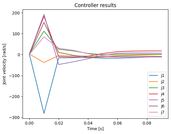

There are three main points that need to be understood about task-space singularities.

singularities have to be addressed so that the robot does not damage itself and things/people in its surroundings,
singularities are a manifestation of mechanical phenomena related to the definition of the task-space. They do not mean the mathematic model is broken, they simply and correctly represent a mechanical issue.
singularities usually occur when joints are aligned, but predicting singular configurations for robots with a large number of degrees-of-freedom is not trivial.

Damped pseudo-inverse¶

The damped pseudo-inverse is an interesting alternative to the SVD-based inverse that gives the system some robustness to task-space singularities. The main idea is to use the following pseudo-inverse for any (possibly singular) matrix $B\in {\mathbb{R}}^{m\times n}$ , called the damped-pseudo inverse

B^+ \triangleq {\left(B^T B+\lambda^2 I\right)}^{-1} B^T

(15)

where $\lambda \in \mathbb{R}-\lbrace 0\rbrace$ is the damping factor. The meaning of this damping factor will become clearer in the next lesson, but for now it suffices to know that given that

{\left(B^T B+\lambda^2 I\right)}^{-1} \:\textrm{(Bonus}\;\textrm{Homework}\;\textrm{2)}

(16)

always exists, regular inversion algorithms can be used to calculate the damped pseudo-inverse. Using MATLAB, this would mean, for instance

B = np.array([[2, 0, 1, 2],
              [0, 0, 1, 4],
              [2, 0, 1, 2]])

λ = 0.01
B_damped_pinv = np.linalg.inv(B.T @ B + (λ ** 2) * np.eye(4)) @ B.T

B @ B_damped_pinv

array([[4.99994097e-01, 6.24984841e-06, 4.99994097e-01],
       [6.24984750e-06, 9.99987500e-01, 6.24984750e-06],
       [4.99994097e-01, 6.24984841e-06, 4.99994097e-01]])

Damped pseudo-inverse and singularity robustness¶

In the point-of-view of Jacobian-based robot control, the damping factor lets us balance the trade-off between optimal joint velocities (in the sense of task error reduction) and joint velocity norm.

If you choose a larger damping factor, the robot will be more robust to task-space singularities, but it might take longer to reach the desired task-space value. As you lower the damping factor, the behavior gets closer to the SVD-based pseudo-inverse. If the damping is too low, the joint velocities will also be dangerous when the robot is close to singular configurations.

To show a concrete example of the damped pseudo-inverse in action, let us copy and paste our prior example. After that, we change only the damping factor and see its effect on robot control.

# Define the robot
seven_dof_planar_robot = SevenDofPlanarRobotDH.kinematics()

# Define the controller
translation_controller = DQ_PseudoinverseController(seven_dof_planar_robot)
translation_controller.set_control_objective(ControlObjective.Translation)
translation_controller.set_gain(10)

damping = 1

translation_controller.set_damping(damping)

# Desired translation (pure quaternion)
td = 7 * j_
# Sampling time [s]
tau = 0.01
# Simulation time [s]
time_final = 1
# Initial joint values [rad]
q = np.zeros(7)
# Store the control signals
stored_u = []
stored_time = []
stored_q = []

# Translation controller loop.
for time in np.arange(0, time_final + tau,tau):
    # Store q for posterior animation
    stored_q.append(q)
    
    # Get the next control signal [rad/s]
    u = translation_controller.compute_setpoint_control_signal(q, vec4(td))

    # Move the robot
    q = q + u * tau

    # Store data
    stored_u.append(u)
    stored_time.append(time)

The behavior can be seen as follows.

fig, ax = setup_plot()
anm.FuncAnimation(fig, 
                  partial(animate_robot, robot=seven_dof_planar_robot, stored_q=stored_q, xd = 1 + 0.5*E_*td), 
                  frames=len(stored_q))

And control signals as follows.

plot_u(np.array(stored_u), np.array(stored_time), 10)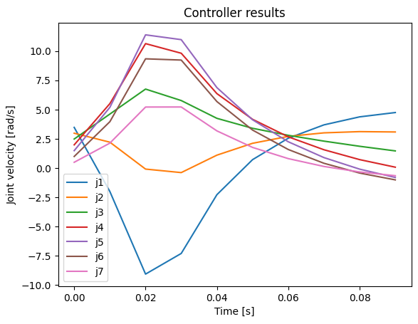

As you can also see from the plotted values, the robot safely moved towards the goal without excessive joint velocities when $\lambda =1$ .

Homework¶

Consider the 7-DoF planar robot used during this lesson. Consider the following damping values $\lambda \in \left\lbrace 0.001,0.01,0.1,0.2,0.3,0.4,0.5,1\right\rbrace$ .

Condition 1: $\theta_i =0$ $\forall$ $i$ to $t_d =7\hat{\jmath}$ . $\eta =10,\tau =0.01$

Create a file called seven_dof_robot_damping_comparison_singular.py that does the following

Run the following nine controllers: one SVD-based pseudoinverse translation controller AND eight damped-pseudo inverse translation controllers, each one with one of the damping values defined above. Store their task-space error norm and their control signal norm.
Using subplot with one row and two columns: plot on the left subplot the task-space error norm for all controllers, so that they can be compared. On the right subplot, plot the control signal norm for all controllers so that they can be compared*.*

Condition 2: $\theta_i =\pi /12$ $\forall$ $i$ to $t_d =7\hat{\jmath}$ . $\eta =10,\tau =0.01$

Create a file called seven_dof_robot_damping_comparison.py that does the following

Run the following nine controllers: one SVD-based pseudoinverse translation controller AND eight damped-pseudo inverse translation controllers, each one with one of the damping values defined above. Store their task-space error norm and their control signal norm.
Using subplot with one row and two columns: plot on the left subplot the task-space error norm for all controllers, so that they can be compared. On the right subplot, plot the control signal norm for all controllers so that they can be compared*.*

Bonus Homework¶

Do the following on pen-and-paper or in your favorite text editor.

Show that $AA^{\dagger} =U{{\Sigma }}V^T V{{{\Sigma }}}^{\textrm{inv}} U^T =I_{m\times m}$ for any matrix $A^{m\times n} ,\textrm{rank}(A)=m$ , $m\le n$ , with other variables as defined in this lesson.
Show that $\left(B^T B+\lambda I\right)$ is always invertible, for any matrix $B^{m\times n} ,\textrm{rank}(B)<m$ , $m\le n$ , with other variables as defined in this lesson.

[Advanced] DQ Robotics

DQ6 Robot Control Basics using DQ Robotics - Part 2

[Advanced] DQ Robotics

DQ8 Optimization-based Robot Control