DQ8 Optimization-based Robot Control¶

I found an issue¶

Thank you! Please report it at https://github.com/MarinhoLab/OpenExecutableBooksRobotics/issues

Introduction¶

In the last lesson, you learned the concept of task-space singularities and a particular way to address them.

In this lesson, we will revisit the topic of robot control using quadratic optimization formalism.

Notation¶

Keep these in mind (we will also use this notation when writing papers for conferences and journals):

• $h\in \mathbb{H}$: a quaternion. (Bold-face, lowercase character)
• $\underline{h} \in \mathcal{H}$: a dual quaternion. (Bold-face, underlined, lowercase character)
• $p,t,\cdots \in {\mathbb{H}}_p$: pure quaternions. They represent points, positions, and translations. They are quaternions for which $\textrm{Re}\left(h\right)=0$.
• $r\in {\mathbb{S}}^3$: unit quaternions. They represent orientations and rotations. They are quaternions for which $||h||=1$.
• $\underline{x} \in \underline{\mathcal{S}}$: unit dual quaternions. They represent poses and pose transformations. They are dual quaternions for which $||h||=1$.
• $\underline{l} \in {\mathcal{H}}_p \cap$ $\underline{{\mathcal{S}}}$ : a Plücker line.
• $\underline{{{\pi }}} \in \left\lbrace P\left(\underline{{{\pi }}} \right)\in {\mathbb{H}}_p \right\rbrace \cap \underline{{\mathcal{S}}}$ : a plane.
• $\theta, a,b,\cdots \in \mathbb{R}$: real numbers.
• ${{q,\cdots }}\in {\mathbb{R}}^n:$ real vectors.
• $J, A, B,\cdots \in {\mathbb{R}}^{m\times n}:$ real matrices.

Robot definition¶

The concepts of this lesson apply to any manipulator robot. However, to have a more concrete understanding using DQ Robotics, consider the same robot as used in the past lesson.

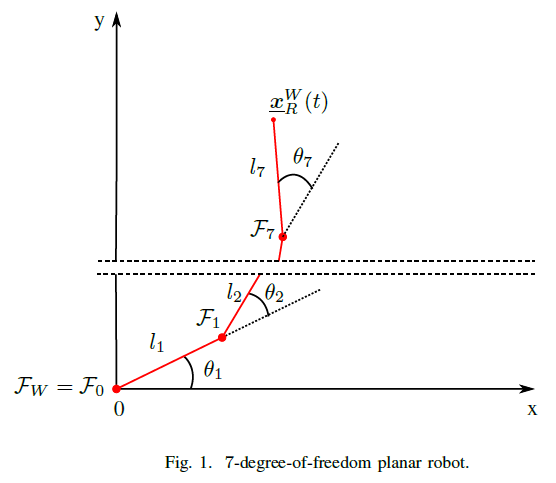
1. Let the robot $R$ be a 7-DoF planar robot, as drawn in Fig.1.
2. Let ${\mathcal{F}}_W$ be the world-reference frame.
3. Let ${\underline{x} }_R^W (t)\triangleq {\underline{x} }_R$ $\in$ $\underline{\mathcal{S}}$ represent the pose of the end effector.
4. Let $R$ be composed of seven rotational joints that rotate about their z-axis, composed in the joint-space vector $q\left(t\right)\triangleq q={\left\lbrack \theta_1 ~\theta_2 ~\theta_3 ~\theta_4 ~\theta_5 ~\theta_6 ~\theta_7 \right\rbrack }^T$ with $\theta_i \left(t\right)\triangleq \theta_i \in \mathbb{R}$ for $i=1,2,\ldots,7$. The rotation of the reference frames of each joint coincides with the rotation of ${\mathcal{F}}_W$ when $\theta_i =0$. The lengths of the joints are $l_i \in$ ${\mathbb{R}}^+ -\lbrace 0\rbrace$.
5. Consider that we can freely control the joint vector $q$.

This robot can be modeled by the following class.

Let us instantiate our robot as follows

A brief review of quadratic optimization¶

At some point in your education, you might have been introduced to optimization problems. There are many types of optimization problems, and in this lesson, we will address only two types, which are enough to solve a large class of robot control problems.

Unconstrained quadratic optimization¶

The first type is called unconstrained quadratic optimization

where $\mathcal{F}\left(\dot{q} \right)\in {\mathbb{R}}^+$ is a quadratic objective function that depends on the current joint configuration. Note that it is called an optimization problem, and NOT an equation (note that there is no equality sign). In mathematical optimization terminology, $\dot{q}$ is called the decision variable.

You can read that as “find all $\dot{q}$ that minimize $\mathcal{F}\left(\dot{q} \right)$ and return one of them as $u$.” The solution for an unconstrained quadratic optimization problem can, in general, be found analytically. In this lesson we will call that minimizer as $u$.

Quadratic programming¶

The second type of optimization problem that we will address is called quadratic programming (QP), which is a linearly constrained quadratic optimization problem, in the form

where $W\in {\mathbb{R}}^{n\times p}$ and $w\in {\mathbb{R}}^p$ represent $p$ linear constraints related to the $n$ degrees-of-freedom of the robot. Note that we use $\preceq$ and not $\le$ because we are representing element-wise inequalities.

You can read that QP as “find all $\dot{q}$ that minimize $\mathcal{F}\left(\dot{q} \right)$, subject to $W\dot{q}$ less or equal to $w$, and return one of them as $u$.” In general, numerical methods are required to obtain a solution for a QP. Similarly to the unconstrained case, in this lesson we will call that minimizer as $u$.

The damped pseudo-inverse as the solution of an unconstrained quadratic optimization problem¶

In the last lesson, the meaning of the damping factor was introduced in the point-of-view of the SVD of the robot’s task Jacobian.

The damping factor can be trivially understood when we re-write the robot control problem in the following way

where $J\in {\mathbb{R}}^{m\times n}$ is the task Jacobian for an $n-$ DoF robot and an $m-$ DoF task. In addition, $\eta \in {\mathbb{R}}^+ -\lbrace 0\rbrace$ is the proportional gain of the controller and $\tilde{x} \in {\mathbb{R}}^m$ is the task error. Lastly, $\lambda \in \mathbb{R}$ is the damping factor.

Note that we are balancing two terms in the objective function. The first term, $||J\dot{q} +\eta \tilde{x} ||^2$, will be high when the task error is high and zero when the task error is zero. The second term, $\lambda^2 ||\dot{q} ||^2$, will penalize high joint velocities depending on the size of the damping factor. As we saw in practice in the last lesson, the damping factor is used as a term to balance task error convergence and the norm of the joint velocities.

Given that we have an unconstrained quadratic optimization problem which is, by definition, convex, the solution is straightforward. The optimum is where the first-order partial derivative of the objective function with respect to the decision variable equals to zero. Hence

Notice that this solution is exactly the same as the damped pseudo-inverse used in the last lesson.

Joint limits¶

Using unconstrained optimization to solve robot-control tasks is useful in some cases, but most tasks in practice have what we call hard limits. They are called that way in the sense that those limits are joint-space or task-space limits that cannot be trespassed. For instance, joint limits are a physical type of hard limit. The controller cannot command the robot to move over its joint limits.

When performing kinematic control, the decision variables are the joint velocities and not the joint positions. Therefore, we need to write the joint limits as a linear inequality that depends on the joint velocities.

Suppose that the lower joint limits are $q^- \in {\mathbb{R}}^n$ and the upper joint limits are $q^+ \in {\mathbb{R}}^n$. The most common way of implementing joint limits using a QP is as follows

where

and

where $\eta_{JL} \in {\mathbb{R}}^+ -\lbrace 0\rbrace$ is a configurable gain. In general, we choose $\eta_{JL} =1$.

The main idea behind this constraint is to constrain the velocity of the joint in the direction of the joint limit.

DQ Robotics Example¶

To solve QPs as described in this lesson using DQ Robotics, use the following class

To solve a QP, you have to choose the numerical solver that will be used by the controller. MATLAB has a solver in its optimization toolbox called “quadprog.” To use it, first instantiate the robot and the solver

and then instantiate the controller and set the control objective, the gain, and the damping factor

Let us define the following joint limits

We define the other control-related variables as in the last lesson.

Plot related code with reusable functions animate_robot and setup_plot.

We can then verify that the joint limits have been kept.

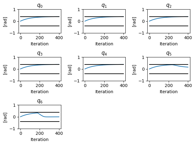
Note that the robot was unable to reach the desired task-space translation due to the joint limits, as shown by the black lines representing the joint limits. This is exactly what we wanted: a controller that will get as close as possible to the target while maintaining the robot’s joint limits.

Vector-field inequalities: task-space collision avoidance¶

We have just now seen how to use linear inequalities to prevent the robot from trespassing on its joint limits. The joint limits are one of the few applications of joint-space constraints. In most cases, we are interested in having task-space constraints. That is, constraints that are defined at the task space. The difficulty in doing so is writing the task-space constraint as linear constraints in joint space.

An effective way of doing so is called vector-field inequalities (VFIs), presented in detail in the following paper.

[1] Marinho, M. M; Adorno, B. V; Harada, K.; and Mitsuishi, M. Dynamic Active Constraints for Surgical Robots using Vector Field Inequalities. IEEE Transactions on Robotics (T-RO), 35(5): 1166–1185. October 2019.

The VFIs are described in detail in [1], so to simplify the discussion for this lesson, consider the (signed) distance $d\triangleq d\left(q\right)\in \mathbb{R}$ to be the relation between some entity in the robot, such as a point, line, or plane, and another entity in the workspace.

Keeping the robot entity outside a restricted zone¶

Consider the situation of keeping the robot entity outside a restricted zone. We define the distance error in such a way that the distance error is positive whenever the robot is outside the restricted zone, zero when at the border, and negative when inside the restricted zone. The distance error is then $\tilde{d} \triangleq d-d_{\textrm{safe}}$, where $d_{\textrm{safe}} \in \mathbb{R}$ is the safe distance, that we suppose to be constant in time in this lesson.

To obtain the general formulation of the VFIs, we start with the following task-space inequality, that will keep our robot outside a restricted zone

where $\eta_d \in {\mathbb{R}}^+ -\lbrace 0\rbrace$ is a proportional gain. To be used in our QP, we need to re-write this as a joint-space linear constraint, which is what the VFI method does.

The VFIs are then given by

Given that the safe distance is constant in time. Now, notice that if the distance depends on the joint values, we can find a distance Jacobian such that the following holds

where $J_d \in {\mathbb{R}}^{1\times n}$ is the distance Jacobian for that specific pair of entities.

The linear constraint for that pair of entities, with respect to the joint velocities, then becomes

That constraint can be re-written to be compatible with our QP definition as

Keeping the robot entity inside a safe zone¶

The reasoning is basically the same of the restricted zone case, but the distance error is redefined as $\tilde{d} \triangleq d_{\textrm{safe}} -d$. This causes the linear constraint to change to

Square distances instead of distances¶

Calculating the distance Jacobians of the distance of some primitives introduces algorithmic singularities, as shown in [2]. To handle that problem, we often calculate the Jacobian of the square distance instead [1]. The notation for square distances is the upper-case letter $D$.

[2] Marinho, M. M; Adorno, B. V; Harada, K.; and Mitsuishi, M. Active Constraints using Vector Field Inequalities for Surgical Robots. In 2018 IEEE International Conference on Robotics and Automation (ICRA), pages 5364–5371, May 2018.

Distance Jacobians¶

In lesson 4, we learned about distance functions using dual quaternions, and in lesson 6 you learned how to calculate a few Jacobians. Using that knowledge, it is easy to calculate the distance Jacobians related to the distance functions.

We will go through how to calculate all the distance Jacobians described in [1] using DQ Robotics, but we will skip most of the mathematical derivations because they are already described in detail in the paper.

Preliminaries¶

To calculate the distance Jacobian, the following two definitions are useful.

First, the cross-product between $a,b\in {\mathbb{H}}_p$ can be mapped into ${\mathbb{R}}^4$ using the operator $\bar{S} \left(.\right)$, as follows [1, Eq. (3)]

${\textrm{vec}}_4 \left(a\times b\right)=\bar{S} \left(a\right){\textrm{vec}}_4 \left(b\right)=\bar{S} {\left(b\right)}^T {\textrm{vec}}_4 \left(a\right)$ ,

Second, the time derivative of the squared norm of a time-varying quaternion $h\left(t\right)\in {\mathbb{H}}_p$ is given by [1, Eq. (4)]

Two new task Jacobians are also needed. Similarly, to how we obtained the translation, rotation, and pose Jacobians, we can also obtain the Jacobians related to lines and planes in the robot.

Line Jacobian¶

Suppose that we want the Jacobian related to line with direction $l_v \in {\mathbb{H}}_p \cap {\mathbb{S}}^3$ that passes through the end-effector. The line will be given by [1, Eq. (24)]

Given our definition of line, we have the following [1, Eq. (28)]

Using DQ Robotics, we can obtain the line Jacobian as follows

where $J_{l_r } \in {\mathbb{R}}^{8\times n}$ is the line Jacobian. It can be decomposed into

where $J_{r_v } \in {\mathbb{R}}^{4\times n}$ is composed of the first four rows of the line Jacobian, which are related to the direction of the line. In addition, $J_{m_v } \in {\mathbb{R}}^{4\times n}$ is composed of the last four rows of the line Jacobian, which are related to the line moment.

Plane Jacobian¶

Lastly, the Jacobian related to the plane in the end-effector with normal $n_{\pi_v } \in {\mathbb{H}}_p \cap {\mathbb{S}}^3$ will be given by

where

and

Point-to-point distance Jacobian¶

Let the translation of the robot’s point entity be $t\left(q\right)\triangleq t\in {\mathbb{H}}_p$ and the position of a point in the workspace be $p\in {\mathbb{H}}_p$. The squared-distance between those two points is, as mentioned in lesson 4, is [1, Eq. (21)]

The derivative of the squared-distance is, therefore [1, Eq. (22)]

This means that the point-to-point distance Jacobian is given by

Using DQ Robotics, it can be calculated as

Point-to-line distance Jacobian¶

Let $\underline{l} \in {\mathcal{H}}_p \cap \underline{{\mathcal{S}}}$ be a line entity in the workspace. The square distance between a point entity in the robot and that line is [1, Eq. (29)]

The point-to-line distance Jacobian is, therefore [1, Eq. (32)]

Using DQ Robotics, it can be calculated as

Line-to-point distance Jacobian¶

Let ${\underline{l} }_v \left(q\right)\triangleq {\underline{l} }_v \in {\mathcal{H}}_p \cap \underline{{\mathcal{S}}}$ be a line entity related to the robot. The square distance between that line and a point in the workspace is given by [1, Eq. (33)]

The line-to-point distance Jacobian is a bit more involved, as described in [1, Eq. (34)].

Using DQ Robotics, it can be calculated as

Line-to-line distance Jacobian¶

Suppose that we want to calculate the Jacobian that relates the distance between a line entity in the robot, ${\underline{l} }_v$, and a line in the workspace $\underline{l} .$ The mathematical derivation is described in detail in [1, Eq. (48)]. To obtain the line-to-line distance Jacobian using DQ Robotics, we do

Point-to-plane distance Jacobian¶

Let $\underline{{{\pi }}} \in \left\lbrace P\left(\underline{{{\pi }}} \right)\in {\mathbb{H}}_p \right\rbrace \cap \underline{{\mathcal{S}}}$ be a plane entity in the workspace. The signed distance between the robot’s translation, $t$, and the plane, in the point of view of the plane is given by [1, Eq. (57)].

The point-to-plane distance Jacobian will therefore be given by [1, Eq. (59)]

Using DQ Robotics, it can be obtained as

Plane-to-point distance Jacobian¶

Let ${\underline{{{\pi }}} }_v \left(q\right)\triangleq {\underline{{{\pi }}} }_v \in \left\lbrace P\left({\underline{{{\pi }}} }_v \right)\in {\mathbb{H}}_p \right\rbrace \cap \underline{{\mathcal{S}}}$ be a plane entity in the robot. The signed distance between the robot’s plane entity, ${\underline{{{\pi }}} }_v$, and a point in the workspace, $p$, in the point of view of the plane is given by [1, Eq. (57)]

The plane-to-point distance Jacobian will be given by

Using DQ Robotics, it can be obtained as

Vector-field inequalities in action¶

We saw how to calculate several types of distances and distance Jacobians. Now we need to put this knowledge to good use.

Preventing collision with walls¶

Suppose that there is one wall above and one wall below our 7-DoF planar robot, and we want to prevent any collisions between the robot and those walls.

The top wall is given by

and the bottom wall is given by

Note that the normals of those planes are pointing towards the robot. This is important because it means that the distance of any point of the robot will be positive with respect to those planes. Mistaking the direction of the plane’s normal is a common error, so be careful.

Let us plot the two walls.

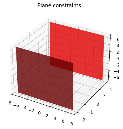
To prevent the collision between the robot and those walls, one strategy is to create one point-to-plane constraint for each of the robot’s joints with respect to those planes. This corresponds to a total of fourteen linear constraints.

Using DQ Robotics, they can be implemented as follows.

Plot related code with reusable functions animate_robot_with_planes and setup_plot.

Entry-sphere constraint¶

A widespread type of constraint in minimally invasive surgery is the entry-sphere constraint. Suppose there is an incision in the skin of the patient, positioned at

Let us define the sphere to have a radius of 0.25 m. That is, we choose

Moreover, let us attach to our planar robot a 2-meter-long shaft whose axis is collinear with the $x-$ axis of the last link, as follows

Let us control the robot to the following desired translation

In a way that the shaft never goes outside the entry-sphere. Using DQ Robotics, this can be done as follows

We define a plot function animate_robot_with_entry_sphere and reuse setup_plot defined earlier.

Homework¶

Create a class called VS050RobotDH that represents the Denso VS050 robot, whose DH parameters are described in the following table and is composed entirely of revolute joints. (Remember lesson 6)

End-effector: attach to the robot a 20cm-long-shaft along the $z-$ axis of the last joint.

Initial configuration: $q(0)={\left\lbrack \begin{array}{cccccc} 0 & \frac{\pi }{3} & \frac{\pi }{3} & 0 & \frac{\pi }{3} & 0 \end{array}\right\rbrack }^T .$

1. Create a file called vs050_plane_constraints.py and do the following:
   1. Create a translation controller with $\tau =0.01$. Choose the other controller parameters so that the control is smooth (see this and prior lessons for examples).
   2. Create 6 planes centered around the point $p_1 =0.45\hat{\imath} +0.08\hat{k}$, so that all normals are pointed inwards, to make a 5 cm cube. (remember lesson 4)
   3. During control, use point-to-plane VFIs to keep the tooltip always inside the cubic region.
   4. Move the end-effector, in order, to the following four desired positions $t_d =\left\lbrace 0.60\hat{\imath} +0.08\hat{k}, 0.20\hat{\imath} +0.15\hat{k}, 0.45\hat{\imath} +0.08\hat{k}, 0.45\hat{\imath} +0.0\hat{k} \right\rbrace$, for 4 simulation-time seconds each.
   5. Plot the task error in one figure
   6. Plot the distance of the end-effector to all the six planes using subplots in another figure.
2. Create a file called vs050_entry_sphere_constraint.py and do the following:
   1. Create a translation controller with $\tau =0.01$. Choose the other controller parameters so that the control is smooth (see this and prior lessons for examples).
   2. Consider the entry-sphere to be centered at $p_2 =0.45\hat{\imath} +0.2\hat{k}$. Consider the entry sphere to have a radius of 5 mm.
   3. During control, use a line-to-point VFI to keep the shaft always inside the entry-sphere.
   4. Move the end-effector, in order, to the following four desired positions $t_d =\left\lbrace 0.45\hat{\imath} +0.03\hat{k}, 0.48\hat{\imath} +0.03\hat{k}, 0.41\hat{\imath} +0.03\hat{k}, 0.40\hat{\imath} +0.01\hat{k} \right\rbrace$, for 4 simulation-time seconds each.
   5. Plot the task error in one figure
   6. Plot the distance of the shaft to the center of the entry-sphere in another figure.