%%capture
'''
(C) Copyright 2020-2025 Murilo Marques Marinho (murilomarinho@ieee.org)

     This file is licensed in the terms of the
     Attribution-NonCommercial-ShareAlike 4.0 International (CC BY-NC-SA 4.0)
     license.

 Derivative work of:
 https://github.com/dqrobotics/learning-dqrobotics-in-matlab/tree/master/robotic_manipulators
 Contributors to this file:
     Murilo Marques Marinho (murilomarinho@ieee.org)
'''
DQ6 Robot Control Basics using DQ Robotics - Part 2
I found an issue
Thank you! Please report it at https://
Introduction
In the last lesson, I introduced you to the basics of kinematic modeling and kinematic control using a 1-DoF planar robot. The main point of that lesson was to teach you how to develop your robots from scratch, if needed.
Nonetheless, the DQ Robotics library has many of those functionalities built-in. In this lesson, you will learn how to model serial manipulators using the Denavit-Hartenberg parameters and how to calculate important Jacobians using DQ Robotics. You will also learn how to create a basic kinematic controller using DQ Robotics.
%%capture
%pip install dqrobotics dqrobotics-pyplot
%pip install dqrobotics dqrobotics-pyplot --break-system-packages
from math import sin, cos
import numpy as np
from dqrobotics import *
from dqrobotics_extensions.pyplot import plot
import matplotlib.pyplot as plt
plt.rcParams["animation.html"] = "jshtml" # Need to output animation's videos
import matplotlib.animation as anm
from functools import partial # Need to call functions correctly for matplotlib animationsIntroduction
In the last lesson, I introduced you to the basics of kinematic modeling and kinematic control using a 1-DoF planar robot. The main point of that lesson was to teach you how to develop your robots from scratch, if needed.
Nonetheless, the DQ Robotics library has many of those functionalities built-in. In this lesson, you will learn how to model serial manipulators using the Denavit-Hartenberg parameters and how to calculate important Jacobians using DQ Robotics. You will also learn how to create a basic kinematic controller using DQ Robotics.
Notation
Keep these in mind (we will also use this notation when writting papers to conferences and journals):
- : a quaternion. (Bold-face, lowercase character)
- : a dual quaternion. (Bold-face, underlined, lowercase character)
- : pure quaternions. They represent points, positions, and translations. They are quaternions for which .
- : unit quaternions. They represent orientations and rotations. They are quaternions for which .
- : unit dual quaternions. They represent poses and pose transformations. They are dual quaternions for which .
- : a Plücker line.
- : a plane.
Problem Definition
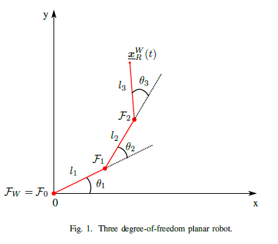
- Let the robot be a 3-DoF planar robot, as drawn in Fig.1.
- Let be the world-reference frame.
- Let represent the pose of the end effector.
- Let be composed of three rotational joints that rotates about their z-axis, composed in the joint-space vector with . The rotation of the reference frames of each joint coincide with the rotation of when . The length of the links are .
- Consider that we can freely control the joint vector .
Problems:
- Obtain the (pose) foward kinematic model of the robot using a set of DH parameters.
- Obtain the pose Jacobian, rotation Jacobian, and translation Jacobian of .
- Using 1. and 2., design a closed-loop pose controller, rotation controller, and translation controller.
Modeling serial robots using Denavit-Hartenberg Parameters
In the last lesson, you modelled a 2-DoF planar robot. As the number of DoF and the complexity of the robots increase, modeling them requires a more general, systematic, and scalable strategy. In this lesson we will show how serial manipulators are modeled using the Denavit-Hartenberg (DH) parameters. This is the standard methodology used in DQ robotics for modeling serial robots.
Forward Kinematic Model using DH parameters
For robots in 3D space, obtaining the robot’s pose transformation is the most generic form of FKM for the end effector. When using unit dual quaternions, retrieving the rotation, translation, etc from the pose is quite straighforward. So let us obtain the pose FKM of the robot using the DH parameters.
Before going into detail about the DH parameters, let be the reference frame at the base of the robot. For convenience, it can coincide with the reference frame of the first joint of the robot.
The first joint enacts a pose transformation from the reference frame of the first joint to the reference frame of the second joint given by
that depends on the joint value of the first joint.
Given that the 3-DoF planar robot has three joints, the robot can be modeled with three consecutive transformations
where and . This sequence of transformation is a methodology that can be used for a serial manipulator with any number of joints.
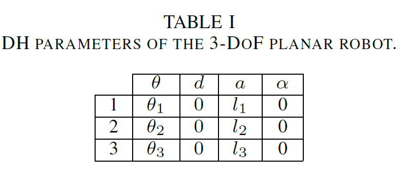
The DH parameters provide a systematic way to calculate each individual joint transformation of any n-DoF serial manipulator. Each joint transformation, , with is composed of four intermediate transformations, as follows
where the DH parameters, for each joint, are . Each of those parameters is related to one transformation. The first is the rotation of about the z-axis of frame
the second is a translation of about the z-axis of frame ,
the third is the translation of about the x-axis of frame ,
the fourth, and last, is the rotation of about the x-axis of frame
Back to our example, the following table summarizes the DH parameters of the 3-DoF planar robot.
DQ Robotics Example
Let us create a class representing the 3-DoF planar robot using DH parameters. The good news is that most of the hard work is handled by DQ Robotics, using the following class
from dqrobotics.robot_modeling import DQ_SerialManipulatorDH
help(DQ_SerialManipulatorDH)
Help on class DQ_SerialManipulatorDH in module dqrobotics._dqrobotics._robot_modeling:
class DQ_SerialManipulatorDH(DQ_SerialManipulator)
| Method resolution order:
| DQ_SerialManipulatorDH
| DQ_SerialManipulator
| DQ_Kinematics
| pybind11_builtins.pybind11_object
| builtins.object
|
| Methods defined here:
|
| __init__(...)
| __init__(self: dqrobotics._dqrobotics._robot_modeling.DQ_SerialManipulatorDH, arg0: typing.Annotated[numpy.typing.ArrayLike, numpy.float64, "[m, n]"]) -> None
|
| get_alphas(...)
| get_alphas(self: dqrobotics._dqrobotics._robot_modeling.DQ_SerialManipulatorDH) -> typing.Annotated[numpy.typing.NDArray[numpy.float64], "[m, 1]"]
|
| Retrieves the vector of alphas.
|
| get_as(...)
| get_as(self: dqrobotics._dqrobotics._robot_modeling.DQ_SerialManipulatorDH) -> typing.Annotated[numpy.typing.NDArray[numpy.float64], "[m, 1]"]
|
| Retrieves the vector of as.
|
| get_ds(...)
| get_ds(self: dqrobotics._dqrobotics._robot_modeling.DQ_SerialManipulatorDH) -> typing.Annotated[numpy.typing.NDArray[numpy.float64], "[m, 1]"]
|
| Retrieves the vector of ds.
|
| get_thetas(...)
| get_thetas(self: dqrobotics._dqrobotics._robot_modeling.DQ_SerialManipulatorDH) -> typing.Annotated[numpy.typing.NDArray[numpy.float64], "[m, 1]"]
|
| Retrieves the vector of thetas.
|
| get_types(...)
| get_types(self: dqrobotics._dqrobotics._robot_modeling.DQ_SerialManipulatorDH) -> typing.Annotated[numpy.typing.NDArray[numpy.float64], "[m, 1]"]
|
| Retrieves the vector of types.
|
| raw_fkm(...)
| raw_fkm(self: dqrobotics._dqrobotics._robot_modeling.DQ_SerialManipulatorDH, arg0: typing.Annotated[numpy.typing.ArrayLike, numpy.float64, "[m, 1]"], arg1: typing.SupportsInt) -> dqrobotics._dqrobotics.DQ
|
| Retrieves the raw FKM.
|
| raw_pose_jacobian(...)
| raw_pose_jacobian(self: dqrobotics._dqrobotics._robot_modeling.DQ_SerialManipulatorDH, arg0: typing.Annotated[numpy.typing.ArrayLike, numpy.float64, "[m, 1]"], arg1: typing.SupportsInt) -> typing.Annotated[numpy.typing.NDArray[numpy.float64], "[m, n]"]
|
| Retrieves the raw pose Jacobian.
|
| raw_pose_jacobian_derivative(...)
| raw_pose_jacobian_derivative(self: dqrobotics._dqrobotics._robot_modeling.DQ_SerialManipulatorDH, arg0: typing.Annotated[numpy.typing.ArrayLike, numpy.float64, "[m, 1]"], arg1: typing.Annotated[numpy.typing.ArrayLike, numpy.float64, "[m, 1]"], arg2: typing.SupportsInt) -> typing.Annotated[numpy.typing.NDArray[numpy.float64], "[m, n]"]
|
| Retrieves the raw pose Jacobian derivative.
|
| ----------------------------------------------------------------------
| Methods inherited from DQ_SerialManipulator:
|
| fkm(...)
| fkm(*args, **kwargs)
| Overloaded function.
|
| 1. fkm(self: dqrobotics._dqrobotics._robot_modeling.DQ_SerialManipulator, arg0: typing.Annotated[numpy.typing.ArrayLike, numpy.float64, "[m, 1]"]) -> dqrobotics._dqrobotics.DQ
|
| Gets the fkm.
|
| 2. fkm(self: dqrobotics._dqrobotics._robot_modeling.DQ_SerialManipulator, arg0: typing.Annotated[numpy.typing.ArrayLike, numpy.float64, "[m, 1]"], arg1: typing.SupportsInt) -> dqrobotics._dqrobotics.DQ
|
| Gets the fkm.
|
| get_dim_configuration_space(...)
| get_dim_configuration_space(self: dqrobotics._dqrobotics._robot_modeling.DQ_SerialManipulator) -> int
|
| Retrieves the number of links.
|
| get_effector(...)
| get_effector(self: dqrobotics._dqrobotics._robot_modeling.DQ_SerialManipulator) -> dqrobotics._dqrobotics.DQ
|
| Retrieves the effector.
|
| get_lower_q_dot_limit(...)
| get_lower_q_dot_limit(self: dqrobotics._dqrobotics._robot_modeling.DQ_SerialManipulator) -> typing.Annotated[numpy.typing.NDArray[numpy.float64], "[m, 1]"]
|
| Retrieves the lower limit for the joint velocities.
|
| get_lower_q_limit(...)
| get_lower_q_limit(self: dqrobotics._dqrobotics._robot_modeling.DQ_SerialManipulator) -> typing.Annotated[numpy.typing.NDArray[numpy.float64], "[m, 1]"]
|
| Retrieves the lower limit for the joint values.
|
| get_upper_q_dot_limit(...)
| get_upper_q_dot_limit(self: dqrobotics._dqrobotics._robot_modeling.DQ_SerialManipulator) -> typing.Annotated[numpy.typing.NDArray[numpy.float64], "[m, 1]"]
|
| Retrieves the upper limit for the joint velocities.
|
| get_upper_q_limit(...)
| get_upper_q_limit(self: dqrobotics._dqrobotics._robot_modeling.DQ_SerialManipulator) -> typing.Annotated[numpy.typing.NDArray[numpy.float64], "[m, 1]"]
|
| Retrieves the upper limit for the joint values.
|
| pose_jacobian(...)
| pose_jacobian(*args, **kwargs)
| Overloaded function.
|
| 1. pose_jacobian(self: dqrobotics._dqrobotics._robot_modeling.DQ_SerialManipulator, arg0: typing.Annotated[numpy.typing.ArrayLike, numpy.float64, "[m, 1]"], arg1: typing.SupportsInt) -> typing.Annotated[numpy.typing.NDArray[numpy.float64], "[m, n]"]
|
| Returns the pose Jacobian
|
| 2. pose_jacobian(self: dqrobotics._dqrobotics._robot_modeling.DQ_SerialManipulator, arg0: typing.Annotated[numpy.typing.ArrayLike, numpy.float64, "[m, 1]"]) -> typing.Annotated[numpy.typing.NDArray[numpy.float64], "[m, n]"]
|
| Returns the pose Jacobian
|
| pose_jacobian_derivative(...)
| pose_jacobian_derivative(*args, **kwargs)
| Overloaded function.
|
| 1. pose_jacobian_derivative(self: dqrobotics._dqrobotics._robot_modeling.DQ_SerialManipulator, arg0: typing.Annotated[numpy.typing.ArrayLike, numpy.float64, "[m, 1]"], arg1: typing.Annotated[numpy.typing.ArrayLike, numpy.float64, "[m, 1]"], arg2: typing.SupportsInt) -> typing.Annotated[numpy.typing.NDArray[numpy.float64], "[m, n]"]
|
| Returns the pose Jacobian derivative
|
| 2. pose_jacobian_derivative(self: dqrobotics._dqrobotics._robot_modeling.DQ_SerialManipulator, arg0: typing.Annotated[numpy.typing.ArrayLike, numpy.float64, "[m, 1]"], arg1: typing.Annotated[numpy.typing.ArrayLike, numpy.float64, "[m, 1]"]) -> typing.Annotated[numpy.typing.NDArray[numpy.float64], "[m, n]"]
|
| Returns the pose Jacobian derivative
|
| set_effector(...)
| set_effector(self: dqrobotics._dqrobotics._robot_modeling.DQ_SerialManipulator, arg0: dqrobotics._dqrobotics.DQ) -> dqrobotics._dqrobotics.DQ
|
| Sets the effector.
|
| set_lower_q_dot_limit(...)
| set_lower_q_dot_limit(self: dqrobotics._dqrobotics._robot_modeling.DQ_SerialManipulator, arg0: typing.Annotated[numpy.typing.ArrayLike, numpy.float64, "[m, 1]"]) -> None
|
| Sets the lower limit for the joint velocities.
|
| set_lower_q_limit(...)
| set_lower_q_limit(self: dqrobotics._dqrobotics._robot_modeling.DQ_SerialManipulator, arg0: typing.Annotated[numpy.typing.ArrayLike, numpy.float64, "[m, 1]"]) -> None
|
| Sets the lower limit for the joint values.
|
| set_upper_q_dot_limit(...)
| set_upper_q_dot_limit(self: dqrobotics._dqrobotics._robot_modeling.DQ_SerialManipulator, arg0: typing.Annotated[numpy.typing.ArrayLike, numpy.float64, "[m, 1]"]) -> None
|
| Sets the upper limit for the joint velocities.
|
| set_upper_q_limit(...)
| set_upper_q_limit(self: dqrobotics._dqrobotics._robot_modeling.DQ_SerialManipulator, arg0: typing.Annotated[numpy.typing.ArrayLike, numpy.float64, "[m, 1]"]) -> None
|
| Sets the upper limit for the joint values.
|
| ----------------------------------------------------------------------
| Methods inherited from DQ_Kinematics:
|
| get_base_frame(...)
| get_base_frame(self: dqrobotics._dqrobotics._robot_modeling.DQ_Kinematics) -> dqrobotics._dqrobotics.DQ
|
| Returns the current base frame
|
| get_reference_frame(...)
| get_reference_frame(self: dqrobotics._dqrobotics._robot_modeling.DQ_Kinematics) -> dqrobotics._dqrobotics.DQ
|
| Returns the current reference frame
|
| set_base_frame(...)
| set_base_frame(self: dqrobotics._dqrobotics._robot_modeling.DQ_Kinematics, arg0: dqrobotics._dqrobotics.DQ) -> None
|
| Sets the base frame
|
| set_reference_frame(...)
| set_reference_frame(self: dqrobotics._dqrobotics._robot_modeling.DQ_Kinematics, arg0: dqrobotics._dqrobotics.DQ) -> None
|
| Sets the reference frame
|
| ----------------------------------------------------------------------
| Static methods inherited from DQ_Kinematics:
|
| distance_jacobian(...) method of builtins.pybind11_detail_function_record_v1_system_libstdcpp_gxx_abi_1xxx_use_cxx11_abi_1 instance
| distance_jacobian(arg0: typing.Annotated[numpy.typing.ArrayLike, numpy.float64, "[m, n]"], arg1: dqrobotics._dqrobotics.DQ) -> typing.Annotated[numpy.typing.NDArray[numpy.float64], "[m, n]"]
|
| Returns the distance Jacobian
|
| distance_jacobian_derivative(...) method of builtins.pybind11_detail_function_record_v1_system_libstdcpp_gxx_abi_1xxx_use_cxx11_abi_1 instance
| distance_jacobian_derivative(arg0: typing.Annotated[numpy.typing.ArrayLike, numpy.float64, "[m, n]"], arg1: typing.Annotated[numpy.typing.ArrayLike, numpy.float64, "[m, n]"], arg2: dqrobotics._dqrobotics.DQ, arg3: typing.Annotated[numpy.typing.ArrayLike, numpy.float64, "[m, 1]"]) -> typing.Annotated[numpy.typing.NDArray[numpy.float64], "[m, n]"]
|
| Returns the distance Jacobian derivative
|
| line_jacobian(...) method of builtins.pybind11_detail_function_record_v1_system_libstdcpp_gxx_abi_1xxx_use_cxx11_abi_1 instance
| line_jacobian(arg0: typing.Annotated[numpy.typing.ArrayLike, numpy.float64, "[m, n]"], arg1: dqrobotics._dqrobotics.DQ, arg2: dqrobotics._dqrobotics.DQ) -> typing.Annotated[numpy.typing.NDArray[numpy.float64], "[m, n]"]
|
| Returns the line Jacobian
|
| line_jacobian_derivative(...) method of builtins.pybind11_detail_function_record_v1_system_libstdcpp_gxx_abi_1xxx_use_cxx11_abi_1 instance
| line_jacobian_derivative(arg0: typing.Annotated[numpy.typing.ArrayLike, numpy.float64, "[m, n]"], arg1: typing.Annotated[numpy.typing.ArrayLike, numpy.float64, "[m, n]"], arg2: dqrobotics._dqrobotics.DQ, arg3: dqrobotics._dqrobotics.DQ, arg4: typing.Annotated[numpy.typing.ArrayLike, numpy.float64, "[m, 1]"]) -> typing.Annotated[numpy.typing.NDArray[numpy.float64], "[m, n]"]
|
| Returns the line Jacobian derivative
|
| line_segment_to_line_segment_distance_jacobian(...) method of builtins.pybind11_detail_function_record_v1_system_libstdcpp_gxx_abi_1xxx_use_cxx11_abi_1 instance
| line_segment_to_line_segment_distance_jacobian(arg0: typing.Annotated[numpy.typing.ArrayLike, numpy.float64, "[m, n]"], arg1: typing.Annotated[numpy.typing.ArrayLike, numpy.float64, "[m, n]"], arg2: typing.Annotated[numpy.typing.ArrayLike, numpy.float64, "[m, n]"], arg3: dqrobotics._dqrobotics.DQ, arg4: dqrobotics._dqrobotics.DQ, arg5: dqrobotics._dqrobotics.DQ, arg6: dqrobotics._dqrobotics.DQ, arg7: dqrobotics._dqrobotics.DQ, arg8: dqrobotics._dqrobotics.DQ) -> typing.Annotated[numpy.typing.NDArray[numpy.float64], "[m, n]"]
|
| Returns the line segment to line segment distance Jacobian
|
| line_to_line_angle_jacobian(...) method of builtins.pybind11_detail_function_record_v1_system_libstdcpp_gxx_abi_1xxx_use_cxx11_abi_1 instance
| line_to_line_angle_jacobian(arg0: typing.Annotated[numpy.typing.ArrayLike, numpy.float64, "[m, n]"], arg1: dqrobotics._dqrobotics.DQ, arg2: dqrobotics._dqrobotics.DQ) -> typing.Annotated[numpy.typing.NDArray[numpy.float64], "[m, n]"]
|
| Returns the line to line angle Jacobian
|
| line_to_line_angle_residual(...) method of builtins.pybind11_detail_function_record_v1_system_libstdcpp_gxx_abi_1xxx_use_cxx11_abi_1 instance
| line_to_line_angle_residual(arg0: dqrobotics._dqrobotics.DQ, arg1: dqrobotics._dqrobotics.DQ, arg2: dqrobotics._dqrobotics.DQ) -> float
|
| Returns the line to line angle residual
|
| line_to_line_distance_jacobian(...) method of builtins.pybind11_detail_function_record_v1_system_libstdcpp_gxx_abi_1xxx_use_cxx11_abi_1 instance
| line_to_line_distance_jacobian(arg0: typing.Annotated[numpy.typing.ArrayLike, numpy.float64, "[m, n]"], arg1: dqrobotics._dqrobotics.DQ, arg2: dqrobotics._dqrobotics.DQ) -> typing.Annotated[numpy.typing.NDArray[numpy.float64], "[m, n]"]
|
| Returns the robot line to line distance Jacobian
|
| line_to_line_residual(...) method of builtins.pybind11_detail_function_record_v1_system_libstdcpp_gxx_abi_1xxx_use_cxx11_abi_1 instance
| line_to_line_residual(arg0: dqrobotics._dqrobotics.DQ, arg1: dqrobotics._dqrobotics.DQ, arg2: dqrobotics._dqrobotics.DQ) -> float
|
| Returns the robot line to line residual
|
| line_to_point_distance_jacobian(...) method of builtins.pybind11_detail_function_record_v1_system_libstdcpp_gxx_abi_1xxx_use_cxx11_abi_1 instance
| line_to_point_distance_jacobian(arg0: typing.Annotated[numpy.typing.ArrayLike, numpy.float64, "[m, n]"], arg1: dqrobotics._dqrobotics.DQ, arg2: dqrobotics._dqrobotics.DQ) -> typing.Annotated[numpy.typing.NDArray[numpy.float64], "[m, n]"]
|
| Returns the robot line to point distance Jacobian
|
| line_to_point_residual(...) method of builtins.pybind11_detail_function_record_v1_system_libstdcpp_gxx_abi_1xxx_use_cxx11_abi_1 instance
| line_to_point_residual(arg0: dqrobotics._dqrobotics.DQ, arg1: dqrobotics._dqrobotics.DQ, arg2: dqrobotics._dqrobotics.DQ) -> float
|
| Returns the robot line to point residual
|
| plane_jacobian(...) method of builtins.pybind11_detail_function_record_v1_system_libstdcpp_gxx_abi_1xxx_use_cxx11_abi_1 instance
| plane_jacobian(arg0: typing.Annotated[numpy.typing.ArrayLike, numpy.float64, "[m, n]"], arg1: dqrobotics._dqrobotics.DQ, arg2: dqrobotics._dqrobotics.DQ) -> typing.Annotated[numpy.typing.NDArray[numpy.float64], "[m, n]"]
|
| Returns the plane Jacobian
|
| plane_jacobian_derivative(...) method of builtins.pybind11_detail_function_record_v1_system_libstdcpp_gxx_abi_1xxx_use_cxx11_abi_1 instance
| plane_jacobian_derivative(arg0: typing.Annotated[numpy.typing.ArrayLike, numpy.float64, "[m, n]"], arg1: typing.Annotated[numpy.typing.ArrayLike, numpy.float64, "[m, n]"], arg2: dqrobotics._dqrobotics.DQ, arg3: dqrobotics._dqrobotics.DQ, arg4: typing.Annotated[numpy.typing.ArrayLike, numpy.float64, "[m, 1]"]) -> typing.Annotated[numpy.typing.NDArray[numpy.float64], "[m, n]"]
|
| Returns the plane Jacobian derivative
|
| plane_to_point_distance_jacobian(...) method of builtins.pybind11_detail_function_record_v1_system_libstdcpp_gxx_abi_1xxx_use_cxx11_abi_1 instance
| plane_to_point_distance_jacobian(arg0: typing.Annotated[numpy.typing.ArrayLike, numpy.float64, "[m, n]"], arg1: dqrobotics._dqrobotics.DQ) -> typing.Annotated[numpy.typing.NDArray[numpy.float64], "[m, n]"]
|
| Returns the robot plane to point distance Jacobian
|
| plane_to_point_residual(...) method of builtins.pybind11_detail_function_record_v1_system_libstdcpp_gxx_abi_1xxx_use_cxx11_abi_1 instance
| plane_to_point_residual(arg0: dqrobotics._dqrobotics.DQ, arg1: dqrobotics._dqrobotics.DQ) -> float
|
| Returns the robot plane to point residual
|
| point_to_line_distance_jacobian(...) method of builtins.pybind11_detail_function_record_v1_system_libstdcpp_gxx_abi_1xxx_use_cxx11_abi_1 instance
| point_to_line_distance_jacobian(arg0: typing.Annotated[numpy.typing.ArrayLike, numpy.float64, "[m, n]"], arg1: dqrobotics._dqrobotics.DQ, arg2: dqrobotics._dqrobotics.DQ) -> typing.Annotated[numpy.typing.NDArray[numpy.float64], "[m, n]"]
|
| Returns the robot point to line distance Jacobian
|
| point_to_line_residual(...) method of builtins.pybind11_detail_function_record_v1_system_libstdcpp_gxx_abi_1xxx_use_cxx11_abi_1 instance
| point_to_line_residual(arg0: dqrobotics._dqrobotics.DQ, arg1: dqrobotics._dqrobotics.DQ, arg2: dqrobotics._dqrobotics.DQ) -> float
|
| Returns the robot point to line residual
|
| point_to_plane_distance_jacobian(...) method of builtins.pybind11_detail_function_record_v1_system_libstdcpp_gxx_abi_1xxx_use_cxx11_abi_1 instance
| point_to_plane_distance_jacobian(arg0: typing.Annotated[numpy.typing.ArrayLike, numpy.float64, "[m, n]"], arg1: dqrobotics._dqrobotics.DQ, arg2: dqrobotics._dqrobotics.DQ) -> typing.Annotated[numpy.typing.NDArray[numpy.float64], "[m, n]"]
|
| Returns the robot point to plane distance Jacobian
|
| point_to_plane_residual(...) method of builtins.pybind11_detail_function_record_v1_system_libstdcpp_gxx_abi_1xxx_use_cxx11_abi_1 instance
| point_to_plane_residual(arg0: dqrobotics._dqrobotics.DQ, arg1: dqrobotics._dqrobotics.DQ) -> float
|
| Returns the robot point to plane residual
|
| point_to_point_distance_jacobian(...) method of builtins.pybind11_detail_function_record_v1_system_libstdcpp_gxx_abi_1xxx_use_cxx11_abi_1 instance
| point_to_point_distance_jacobian(arg0: typing.Annotated[numpy.typing.ArrayLike, numpy.float64, "[m, n]"], arg1: dqrobotics._dqrobotics.DQ, arg2: dqrobotics._dqrobotics.DQ) -> typing.Annotated[numpy.typing.NDArray[numpy.float64], "[m, n]"]
|
| Returns the robot point to point distance Jacobian
|
| point_to_point_residual(...) method of builtins.pybind11_detail_function_record_v1_system_libstdcpp_gxx_abi_1xxx_use_cxx11_abi_1 instance
| point_to_point_residual(arg0: dqrobotics._dqrobotics.DQ, arg1: dqrobotics._dqrobotics.DQ, arg2: dqrobotics._dqrobotics.DQ) -> float
|
| Returns the robot point to point residual
|
| rotation_jacobian(...) method of builtins.pybind11_detail_function_record_v1_system_libstdcpp_gxx_abi_1xxx_use_cxx11_abi_1 instance
| rotation_jacobian(arg0: typing.Annotated[numpy.typing.ArrayLike, numpy.float64, "[m, n]"]) -> typing.Annotated[numpy.typing.NDArray[numpy.float64], "[m, n]"]
|
| Returns the rotation Jacobian
|
| rotation_jacobian_derivative(...) method of builtins.pybind11_detail_function_record_v1_system_libstdcpp_gxx_abi_1xxx_use_cxx11_abi_1 instance
| rotation_jacobian_derivative(arg0: typing.Annotated[numpy.typing.ArrayLike, numpy.float64, "[m, n]"]) -> typing.Annotated[numpy.typing.NDArray[numpy.float64], "[m, n]"]
|
| Returns the rotation Jacobian derivative
|
| translation_jacobian(...) method of builtins.pybind11_detail_function_record_v1_system_libstdcpp_gxx_abi_1xxx_use_cxx11_abi_1 instance
| translation_jacobian(arg0: typing.Annotated[numpy.typing.ArrayLike, numpy.float64, "[m, n]"], arg1: dqrobotics._dqrobotics.DQ) -> typing.Annotated[numpy.typing.NDArray[numpy.float64], "[m, n]"]
|
| Returns the translation Jacobian
|
| translation_jacobian_derivative(...) method of builtins.pybind11_detail_function_record_v1_system_libstdcpp_gxx_abi_1xxx_use_cxx11_abi_1 instance
| translation_jacobian_derivative(arg0: typing.Annotated[numpy.typing.ArrayLike, numpy.float64, "[m, n]"], arg1: typing.Annotated[numpy.typing.ArrayLike, numpy.float64, "[m, n]"], arg2: dqrobotics._dqrobotics.DQ, arg3: typing.Annotated[numpy.typing.ArrayLike, numpy.float64, "[m, 1]"]) -> typing.Annotated[numpy.typing.NDArray[numpy.float64], "[m, n]"]
|
| Returns the translation Jacobian derivative
|
| ----------------------------------------------------------------------
| Static methods inherited from pybind11_builtins.pybind11_object:
|
| __new__(*args, **kwargs) class method of pybind11_builtins.pybind11_object
| Create and return a new object. See help(type) for accurate signature.
Let us represent our robot in the following way, for .
from three_dof_planar_robot_dh import ThreeDofPlanarRobotDH
help(ThreeDofPlanarRobotDH.kinematics)
Help on function kinematics in module three_dof_planar_robot_dh:
kinematics()
Returns the kinematics of the ThreeDoFPlanarRobot as DQ_SerialManipulatorDH.
Note that we use
## This isn't currently exposed in Python and will be fixed in the next release
# DQ_SerialManipulatorDH.JOINT_ROTATIONAL;
to define a rotational joint, so we do not explicilty define in our model.
To calculate the forward kinematics model and plot the robot model, we can simply call the methods already available in the class, as follows
# Initial joint values [rad]
theta1 = -0.1
theta2 = 0.55
theta3 = -1.02

# Joint vector
q = [theta1, theta2, theta3]

# Instantiate the robot kinematics
three_dof_planar_robot = ThreeDofPlanarRobotDH.kinematics()

# Get the fkm, based on theta
x_r = three_dof_planar_robot.fkm(q)

# Plot the robot
plt.figure()
ax = plt.axes(projection='3d')
ax.set_proj_type('ortho')
ax.view_init(azim=0, elev=90) #https://stackoverflow.com/questions/33084853/set-matplotlib-view-to-be-normal-to-the-x-y-plane-in-python
plt.xlabel('x [m]')
plt.ylabel('y [m]')
ax.set_zticks([])
plot(three_dof_planar_robot, q=q)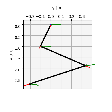
For more details about the methods, check the documentation of the class using
help(DQ_SerialManipulatorDH.fkm)Help on instancemethod in module dqrobotics._dqrobotics._robot_modeling:
fkm(...)
fkm(*args, **kwargs)
Overloaded function.
1. fkm(self: dqrobotics._dqrobotics._robot_modeling.DQ_SerialManipulator, arg0: typing.Annotated[numpy.typing.ArrayLike, numpy.float64, "[m, 1]"]) -> dqrobotics._dqrobotics.DQ
Gets the fkm.
2. fkm(self: dqrobotics._dqrobotics._robot_modeling.DQ_SerialManipulator, arg0: typing.Annotated[numpy.typing.ArrayLike, numpy.float64, "[m, 1]"], arg1: typing.SupportsInt) -> dqrobotics._dqrobotics.DQ
Gets the fkm.
help(plot)Help on function plot in module dqrobotics_extensions.pyplot._pyplot:
plot(obj, **kwargs)
An aggregator for all plot functions related to dqrobotics. Currently, supports `DQ` and `DQ_SerialManipulator`.
Import it as follows:
import dqrobotics_extensions.pyplot as dqp
Before this can be used, please remember to initialise the plt Axes. Example:
plt.figure()
ax = plt.axes(projection='3d')
dqp.plot(i_)
plt.show()
Plotting a unit DQ `x` (See internal function `pyplot._pyplot._plot_pose`):
dqp.plot(x)
Plotting a line DQ `l_dq` (See internal function `pyplot._pyplot._plot_line`):
dqp.plot(l_dq, line=True)
Plotting a plane DQ `pi_dq` (See internal function `pyplot._pyplot._plot_plane`):
dqp.plot(pi_dq, plane=True)
Plotting a `DQ_SerialManipulator` called `robot` at joint configurations `q` (See internal function `pyplot._pyplot._plot_serial_manipulator`):
dqp.plot(robot, q=q)
:param obj: The input to be plotted.
:param kwargs: For arguments depending on the type of plot you need, see the description above.
:raises RuntimeError: If the input instance `obj` has no meaning for function, or if the `obj` is not valid for the input options.
Differential Kinematics Model using DH parameters
Similar to how we calculated the the DKM in the last lesson, the DKM can be calculated for any set of DH parameters.
Pose Jacobian
Using the FKM, we find
where is the pose Jacobian. We do not need to worry about the details of how to calculate this for now. The details of how to calculate the Jacobian for any serial manipulator are described from Page 38 of
ADORNO, B. V., Two-arm manipulation: from manipulators to enhanced human-robot collaboration [Contribution à la manipulation à deux bras : des manipulateurs à la collaboration homme-robot], Université Montpellier 2, Montpellier, France, 2011. (pdf)
Rotation Jacobian
The goal of this section is to find the rotation Jacobian, , so that the following relation holds
The rotation Jacobian is useful to control the rotation of the end effector and can be used to calculate many other Jacobians.
We can conveniently find the rotation Jacobian using the pose Jacobian. To do so, remember that the robot’s end-effector pose can be decomposed as follows
That means that the first-order time-derivative is
that can be re-written as
which means that the pose Jacobian can be decomposed as
Notice that
which means that the rotation Jacobian is . That is, the rotational Jacobian is composed of the first four rows of the pose Jacobian.
Translation Jacobian
The goal of this section is to find the translation Jacobian, , so that the following relation holds
The translation Jacobian is useful to control the translation of the end effector and can be used to calculate many other Jacobians. We can conveniently find the translation Jacobian using the pose Jacobian and the end-effector’s pose.
We start from the translation relation
hence
DQ Robotics Example
The pose Jacobian can be computed using the DQ_SerialManipulatorDH class as follows.
# Get the pose Jacobian
Jx = three_dof_planar_robot.pose_jacobian(q)
The rotation Jacobian and translation Jacobian can be calculated using methods of its DQ_Kinematics superclass. For instance, the rotation Jacobian can be obtained as
# Get the rotation Jacobian, based on the pose Jacobian
Jr = three_dof_planar_robot.rotation_jacobian(Jx)
and the translation Jacobian can be obtained as
# Get the end-effector's pose
x = three_dof_planar_robot.fkm(q)
# Get the translation Jacobian
Jt = three_dof_planar_robot.translation_jacobian(Jx,x)
Task-space position control
In the last lesson you were introduced to the basics of robot control using the inverse differential kinematics model.
Instead of building the controller from scratch, you can use controllers already available in DQ Robotics.
Pseudo-Inverse Controller
In the last lesson, we implemented a simple pseudo-inverse-based kinematic controller. Let us revisit this topic using DQ Robotics.
from dqrobotics.robot_control import DQ_PseudoinverseController
from dqrobotics.robot_control import ControlObjective
Preliminaries
Let us start with the initial conditions of the problem.
Define the sampling time and how many seconds of control we will simulate.
# Sampling time [s]
tau = 0.01
# Simulation time [s]
time_final = 1
Define the initial robot posture.
# Initial joint values [rad]
theta1 = -0.4
theta2 = 1.71
theta3 = 0.85
# Arrange the joint values in a column vector
q_init = [theta1, theta2, theta3]# Desired translation components [m]
tx = 1.25
ty = 1.25
# Desired translation
td = tx*i_ + ty*j_then, the desired rotation.
# Desired rotation component [rad]
gamma = 0.49
# Desired rotation
rd = cos(gamma/2.0) + k_*sin(gamma/2.0)
The desired pose will then be
# Desired pose
xd = rd + 0.5*E_*td*rd
We then instantiate the robot kinematics, as follows.
# Create robot
three_dof_planar_robot = ThreeDofPlanarRobotDH.kinematics()
Translation Controller
The basic syntax to instantiate a translation controller is as follows.
The robot will align the end-effector translation with the desired translation. The rotation is not controlled.
# Instanteate the controller
translation_controller = DQ_PseudoinverseController(three_dof_planar_robot)
translation_controller.set_control_objective(ControlObjective.Translation)
translation_controller.set_gain(5.0)
translation_controller.set_damping(0) # Damping was not explained yet, set it as 0 to use pinv()

# Translation controller loop.
q = q_init
stored_q = []
for time in np.arange(0, time_final + tau,tau):
    # Store q for posterior animation
    stored_q.append(q)

    # Get the next control signal [rad/s]
    u = translation_controller.compute_setpoint_control_signal(q, vec4(td))

    # Move the robot
    q = q + u * tau
Plot related code with reusable functions animate_robot and setup_plot.
# Animation function
def animate_robot(n, robot, stored_q, xd):
    plt.cla()
    plot(robot, q=stored_q[n])
    plot(xd)
    plt.xlabel('x [m]')
    plt.xlim([-0.3, 2])
    plt.ylabel('y [m]')
    plt.ylim([-2, 2])
    ax = plt.gca()
    ax.axes.zaxis.set_ticklabels([])
    plt.title(f'Translation control time={time} s out of {time_final} s')

def setup_plot():
    fig = plt.figure()
    ax = plt.axes(projection='3d')
    ax.set_proj_type('ortho')
    ax.view_init(azim=0, elev=90) #https://stackoverflow.com/questions/33084853/set-matplotlib-view-to-be-normal-to-the-x-y-plane-in-python
    return fig, ax

fig, ax = setup_plot()
anm.FuncAnimation(fig,
                  partial(animate_robot, robot=three_dof_planar_robot, stored_q=stored_q, xd=xd),
frames=len(stored_q))Rotation Controller
The basic syntax to instantiate a rotation controller is as follows.
The robot will align the end-effector rotation with the desired rotation. The translation is not controlled.
# Instantiate the controller
translation_controller = DQ_PseudoinverseController(three_dof_planar_robot)
translation_controller.set_control_objective(ControlObjective.Rotation)
translation_controller.set_gain(5.0)
translation_controller.set_damping(0) # Damping was not explained yet, set it as 0 to use pinv()

# Rotation controller loop.
q = q_init
stored_q = []
for time in np.arange(0, time_final + tau,tau):
    # Store q for posterior animation
    stored_q.append(q)

    # Get the next control signal [rad/s]
    u = translation_controller.compute_setpoint_control_signal(q, vec4(rd));

    # Move the robot
    q = q + u * tau
The behavior can be seen as follows.
# Plot
fig, ax = setup_plot()
anm.FuncAnimation(fig,
                  partial(animate_robot, robot=three_dof_planar_robot, stored_q=stored_q, xd=xd),
frames=len(stored_q))Pose Controller
The basic syntax to instantiate a pose controller is as follows.
The robot will align the end-effector pose with the desired pose. If the rotation and translation cannot be achieved simulatenously, the robot will balance rotation and translation error, according to the controller definitions.
# Instantiate the controller
translation_controller = DQ_PseudoinverseController(three_dof_planar_robot)
translation_controller.set_control_objective(ControlObjective.Pose)
translation_controller.set_gain(5.0)
translation_controller.set_damping(0) # Damping was not explained yet, set it as 0 to use pinv()

# Translation controller loop.
q = q_init
stored_q = []
for time in np.arange(0, time_final + tau,tau):
    # Store q for posterior animation
    stored_q.append(q)

    # Get the next control signal [rad/s]
    u = translation_controller.compute_setpoint_control_signal(q, vec8(xd))

    # Move the robot
    q = q + u * tau
The behavior can be seen as follows.
# Plot
fig, ax = setup_plot()
anm.FuncAnimation(fig,
                  partial(animate_robot, robot=three_dof_planar_robot, stored_q=stored_q, xd=xd),
frames=len(stored_q))Homework
(1) Following the format of ThreeDofPlanarRobotDH.py, create a class called NDofPlanarRobotDH.py as shown in the figure.
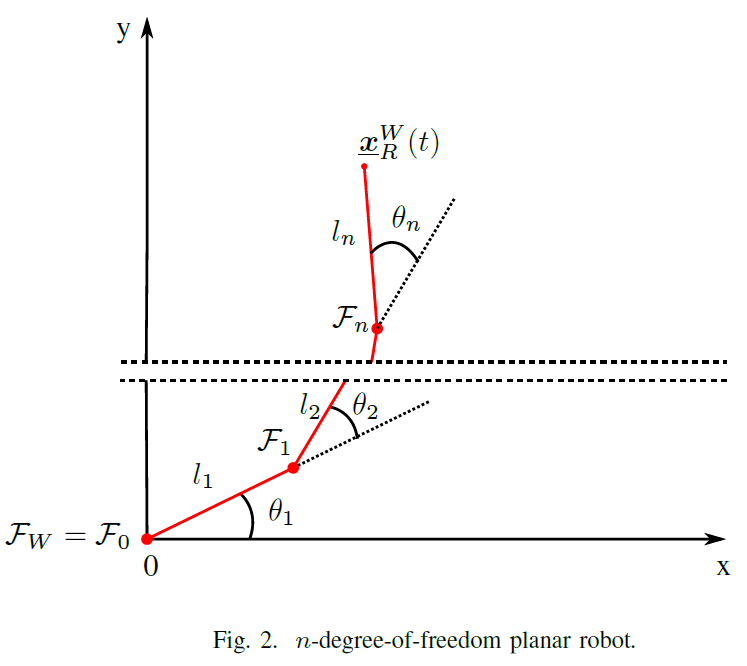
The class must
- Consider all lengths of the links as unitary. That is, .
- Have a “kinematics” method that takes the desired number of DoFs as input and returns the corresponding
DQ_SerialManipulatorDHinstance.
(2) Consider the desired translation , desired rotation , and initial posture for . Use the class you created in (1) to instantiate a 7-DoF planar robot.
- create a script called
seven_dof_planar_robot_translation_control.mthat implements a task-space translation controller using a DQ_PseudoinverseController. Control the 7-DoF planar robot to - create a script called
seven_dof_planar_robot_rotation_control.mthat implements a task-space rotation controller using a DQ_PseudoinverseController. Control the 7-DoF planar robot to - create a script called
seven_dof_planar_robot_pose_control.mthat implements a task-space pose controller using a DQ_PseudoinverseController. Control the 7-DoF planar robot to .