Gallery
Sample plots generated with the latest version of the library directly from the code when the documentation is built.
Images
Preamble
Auxiliar methods pyplot.gallery._utils._set_plot_labels() and pyplot.gallery._utils._set_plot_limits()
are used to make the gallery code uniform.
from matplotlib import pyplot as plt

def _set_plot_labels():
    ax = plt.gca()
    ax.set(
        xlabel='x [m]',
        ylabel='y [m]',
        zlabel='z [m]'
    )

def _set_plot_limits(lmin: float = -0.5, lmax: float = 0.5):
    ax = plt.gca()
    ax.set(
        xlim=[lmin, lmax],
        ylim=[lmin, lmax],
        zlim=[lmin, lmax]
    )
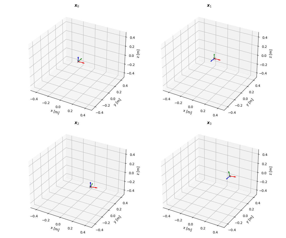
Poses
Generated by
from dqrobotics import *

# Adding the prefix `dqp` to help users differentiate from `plt`
import dqrobotics_extensions.pyplot as dqp
from ._utils import _set_plot_labels, _set_plot_limits

from matplotlib import pyplot as plt

from math import sin, cos, pi

def output_poses():
    """
    Calculate and visualize multiple poses represented as DQs.
    """

    # x1
    t1 = 0
    r1 = 1
    x1 = r1 + 0.5 * E_ * t1 * r1

    # x2
    t2 = 0.1 * j_
    r2 = cos(pi / 4) + i_ * sin(pi / 4)
    x2 = r2 + 0.5 * E_ * t2 * r2

    # x3
    t3 = - 0.1 * k_ + 0.2 * i_
    r3 = cos(pi / 32) + k_ * sin(pi / 32)
    x3 = r3 + 0.5 * E_ * t3 * r3

    # x4
    x4 = x1 * x2 * x3

    # Plot using subplot
    fig = plt.figure(figsize=(12, 10))

    pose_list = [x1, x2, x3, x4]

    for i in range(0, len(pose_list)):
        x = pose_list[i]

        ax = plt.subplot(2, 2, i+1, projection='3d')
        dqp.plot(x)
        ax.title.set_text(rf'$\boldsymbol{{x}}_{i}$')
        _set_plot_labels()
        _set_plot_limits()

    fig.tight_layout()
    plt.savefig("output_poses.png")
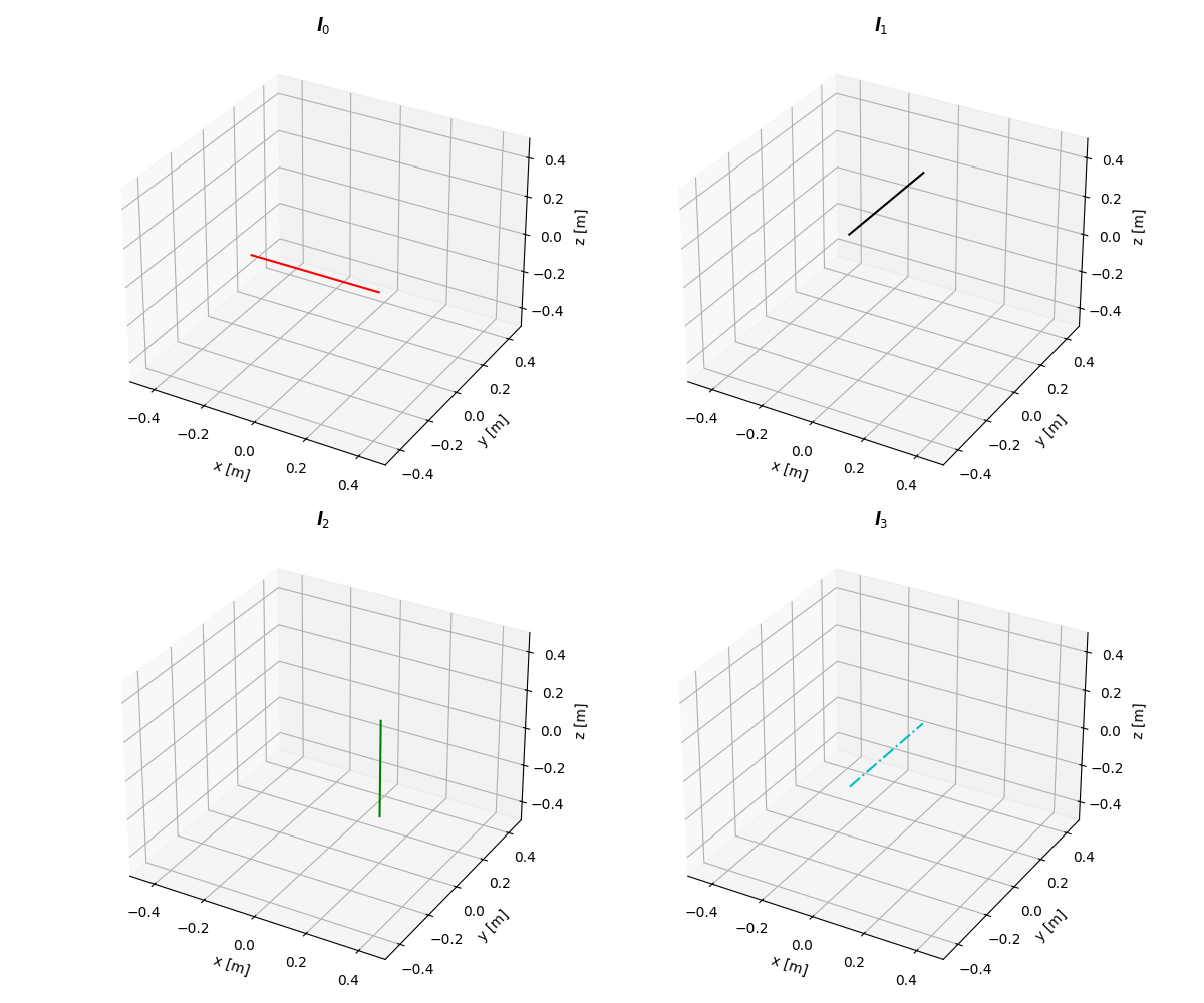
Lines
Generated by
from dqrobotics import *

# Adding the prefix `dqp` to help users differentiate from `plt`
import dqrobotics_extensions.pyplot as dqp
from ._utils import _set_plot_labels, _set_plot_limits

from matplotlib import pyplot as plt


def output_lines():
    """
    Calculate and visualize multiple lines represented as DQs.
    """

    # l1
    l1 = i_
    m1 = cross(-0.1 * j_, l1)
    l1_dq = l1 + E_ * m1

    # l2
    l2 = j_
    m2 = cross(0.3 * k_, l2)
    l2_dq = l2 + E_ * m2

    # l3
    l3 = k_
    m3 = cross(0.2 * i_, l3)
    l3_dq = l3 + E_ * m3

    # l4
    l4 = j_
    m4 = 0
    l4_dq = l4 + E_ * m4

    # Plot using subplot
    fig = plt.figure(figsize=(12, 10))

    line_list = [l1_dq, l2_dq, l3_dq, l4_dq]
    color_list = ['r-', 'k-', 'g-', 'c-.']

    for i in range(0, len(line_list)):
        l_dq = line_list[i]
        color = color_list[i]

        ax = plt.subplot(2, 2, i+1, projection='3d')
        dqp.plot(l_dq, line=True, scale=0.5, color=color)
        ax.title.set_text(rf'$\boldsymbol{{l}}_{i}$')
        _set_plot_labels()
        _set_plot_limits()

    fig.tight_layout()
    plt.savefig("output_lines.png")
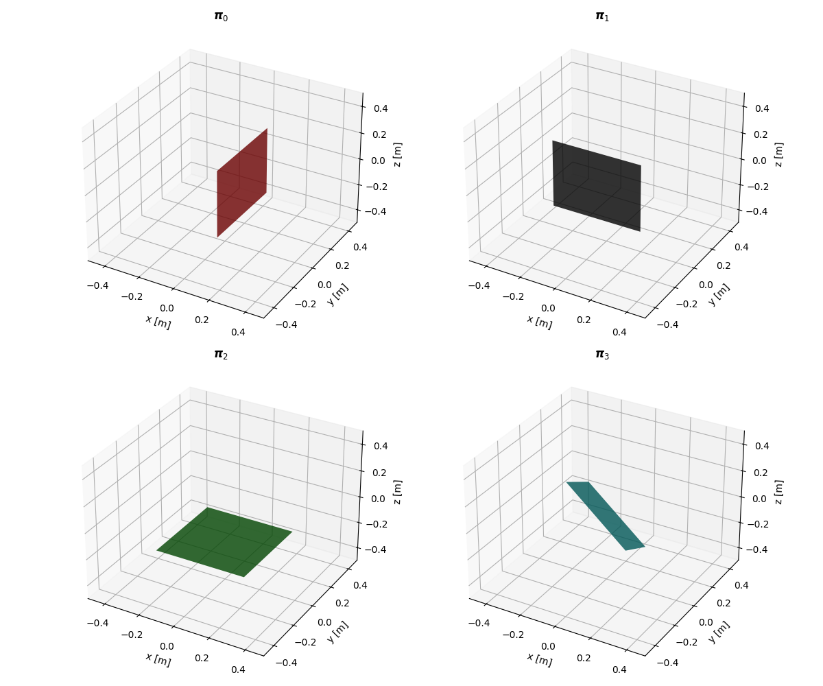
Planes
Generated by
from dqrobotics import *

# Adding the prefix `dqp` to help users differentiate from `plt`
import dqrobotics_extensions.pyplot as dqp
from ._utils import _set_plot_labels, _set_plot_limits

from matplotlib import pyplot as plt


def output_planes():
    """
    Calculate and visualize multiple planes represented as DQs.
    """

    # pi1
    n1_pi = i_
    d1_pi = 0.1
    pi1_dq = n1_pi + E_ * d1_pi

    # pi2
    n2_pi = j_
    d2_pi = -0.1
    pi2_dq = n2_pi + E_ * d2_pi

    # pi3
    n3_pi = -k_
    d3_pi = 0.2
    pi3_dq = n3_pi + E_ * d3_pi

    # pi4
    n4_pi = normalize(i_ + j_ + k_)
    d4_pi = 0
    pi4_dq = n4_pi + E_ * d4_pi

    # Plot using subplot
    fig = plt.figure(figsize=(12, 10))

    plane_list = [pi1_dq, pi2_dq, pi3_dq, pi4_dq]
    color_list = ['r', 'k', 'g', 'c']

    for i in range(0, len(plane_list)):
        pi_dq = plane_list[i]
        color = color_list[i]

        ax = plt.subplot(2, 2, i+1, projection='3d')
        dqp.plot(pi_dq, plane=True, scale=0.5, color=color)
        ax.title.set_text(rf'$\boldsymbol{{\pi}}_{i}$')
        _set_plot_labels()
        _set_plot_limits()

    fig.tight_layout()
    plt.savefig("output_planes.png")
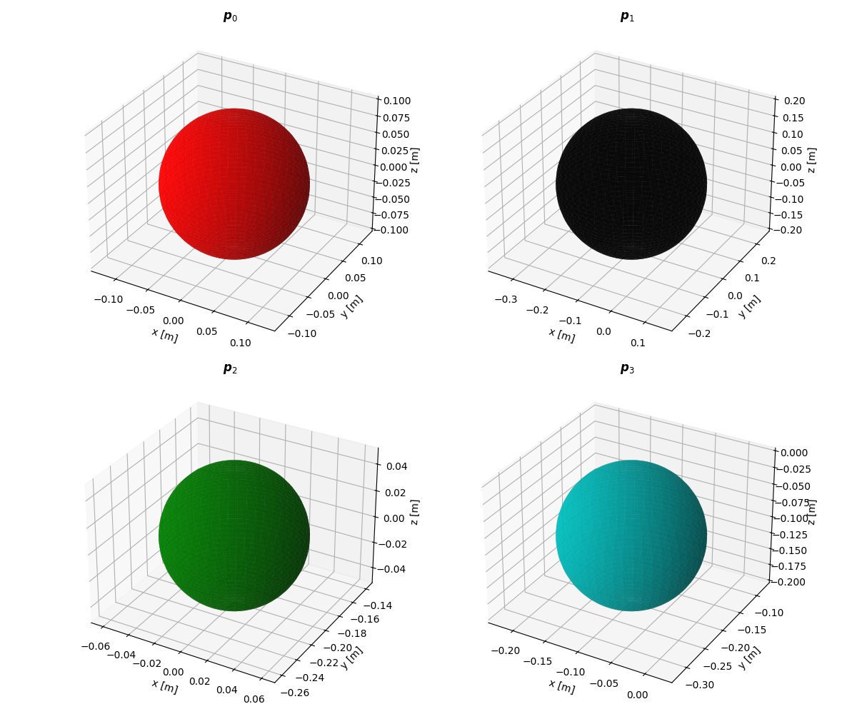
Spheres
Generated by
from dqrobotics import *

# Adding the prefix `dqp` to help users differentiate from `plt`
import dqrobotics_extensions.pyplot as dqp
from ._utils import _set_plot_labels, _set_plot_limits

from matplotlib import pyplot as plt

def output_spheres():
    """
    Calculate and visualize multiple spheres represented as DQs.
    """

    # p1
    p1 = DQ([0])
    r1 = 0.1

    # l2
    p2 = 0.1*i_
    r2 = 0.2

    # l3
    p3 = 0.2*j_
    r3 = 0.05

    # l4
    p4 = 0.1*i_ + 0.2*j_ + 0.1*k_
    r4 = 0.1

    # Plot using subplot
    fig = plt.figure(figsize=(12, 10))

    sphere_list = [(p1, r1), (p2, r2), (p3, r3), (p4, r4)]
    color_list = ['r', 'k', 'g', 'c']

    for i in range(0, len(sphere_list)):
        p, r = sphere_list[i]
        color = color_list[i]

        ax = plt.subplot(2, 2, i + 1, projection='3d')

        dqp.plot(p, sphere=True, radius=r, color=color)

        ax.title.set_text(rf'$\boldsymbol{{p}}_{i}$')
        _set_plot_labels()
        # https://matplotlib.org/stable/gallery/subplots_axes_and_figures/axis_equal_demo.html
        ax.axis('equal') # Adjusted to show that they are spheres not ellipsoids

    fig.tight_layout()
    plt.savefig("output_spheres.png")
Videos
Moving primitives
Generated by
from dqrobotics import *

# Adding the prefix `dqp` to help users differentiate from `plt`
import dqrobotics_extensions.pyplot as dqp
from ._utils import _set_plot_labels, _set_plot_limits

from matplotlib import pyplot as plt
import matplotlib.animation as anm # Matplotlib animation
from functools import partial # Need to call functions correctly for matplotlib animations

from math import sin, cos
import numpy as np


def output_moving_primitives():
    """
    Calculate and visualize multiple moving primitives represented as DQs.
    """

    # Sampling time [s]
    tau = 0.01
    # Simulation time [s]
    time_final = 1
    # Store the plotted variables
    stored_x = []
    stored_l_dq = []
    stored_pi_dq = []
    stored_time = []

    x = DQ([1])
    ls_dq_init = [i_, j_, k_]
    pis_dq_init = [k_, normalize(i_ + j_), normalize(i_ + j_ + k_)]

    # Translation controller loop.
    for time in np.arange(0, time_final + tau, tau):

        # Modify line
        ls_dq = [Ad(x, l_dq_init) for l_dq_init in ls_dq_init]
        pis_dq = [Adsharp(x, pi_dq_init) for pi_dq_init in pis_dq_init]

        # Store data for posterior animation
        stored_x.append(x)
        stored_l_dq.append(ls_dq)
        stored_pi_dq.append(pis_dq)
        stored_time.append(time)

        # Move x
        r = cos((10 * time) / 2) + j_ * sin((10 * time) / 2)
        t = 0.1*(i_ + j_ + k_) * sin(time)
        x = r + 0.5 * E_ * t * r

    def animate_plot(n, stored_x, stored_l_dq, stored_pi_dq, stored_time):

        plt.cla()
        _set_plot_limits()
        _set_plot_labels()
        plt.title(f'Animation time={stored_time[n]:.2f} s out of {stored_time[-1]:.2f} s')

        dqp.plot(stored_x[n])

        line_colors = ['r+-', 'k.-', 'g+-', 'c-.']
        plane_colors = ['r', 'k', 'g', 'c']

        for line_counter in range(len(stored_l_dq[n])):
            l_dq = stored_l_dq[n][line_counter]
            dqp.plot(l_dq, line=True, scale=1, color=line_colors[line_counter % len(line_colors)])
        for plane_counter in range(len(stored_pi_dq[n])):
            pi_dq = stored_pi_dq[n][plane_counter]
            dqp.plot(pi_dq, plane=True, scale=1, color=plane_colors[plane_counter % len(plane_colors)], alpha=0.2)

    # Set up the plot
    fig = plt.figure(dpi=200, figsize=(12, 10))
    plt.axes(projection='3d')

    anim = anm.FuncAnimation(fig,
                      partial(animate_plot,
                              stored_x=stored_x,
                              stored_l_dq=stored_l_dq,
                              stored_pi_dq=stored_pi_dq,
                              stored_time=stored_time),
                      frames=len(stored_x))

    anim.save("output_moving_primitives.mp4")
Moving DQ_SerialManipulator s
Generated by
from dqrobotics import *

# Adding the prefix `dqp` to help users differentiate from `plt`
import dqrobotics_extensions.pyplot as dqp
from dqrobotics.robots import KukaLw4Robot
from dqrobotics.utils.DQ_Math import deg2rad

from ._utils import _set_plot_labels, _set_plot_limits

from matplotlib import pyplot as plt
import matplotlib.animation as anm # Matplotlib animation
from functools import partial # Need to call functions correctly for matplotlib animations

import numpy as np

from math import pi, cos, sin


def output_moving_manipulators():
    """
    Calculate and visualize multiple moving primitives represented as DQs.
    """

    # Animation function
    def animate_robots(n, robots, stored_qs, stored_time):
        """
        Create an animation function compatible with `plt`.
        Adapted from https://marinholab.github.io/OpenExecutableBooksRobotics//lesson-dq8-optimization-based-robot-control.
        :param n: The frame number, necessary for `pyplot`.
        :param robots: The `DQ_SerialManipulator` tuple instance to plot.
        :param stored_qs: The sequence of joint configurations.
        :param stored_time: The sequence of timepoints to plot in the title.
        """
        plt.cla()
        _set_plot_limits(-0, 1.0)
        _set_plot_labels()
        plt.title(f'Joint control time={stored_time[n]:.2f} s out of {stored_time[-1]:.2f} s')

        R1, R2 = robots
        dqp.plot(R1, q=stored_qs[n][0],
                 line_color='r',
                 line_width=5,
                 cylinder_color="k",
                 cylinder_alpha=0.9,
                 cylinder_radius=0.035,
                 cylinder_height=0.1)
        dqp.plot(R2, q=stored_qs[n][1],
                 line_color='b',
                 cylinder_color="c",
                 cylinder_alpha=0.3)

    # Define the robots
    R1 = KukaLw4Robot.kinematics()
    R1.set_reference_frame(cos(pi/2) + k_*sin(pi/2))
    R2 = KukaLw4Robot.kinematics()
    R2.set_reference_frame(1 + 0.5*E_*(0.75*i_ + 0.75*j_))

    # Sampling time [s]
    tau = 0.01
    # Simulation time [s]
    time_final = 1
    # Initial joint values [rad]
    q1 = deg2rad([0, 45, 0, -45, 0, 45, 0])
    q2 = q1
    # Store the control signals
    stored_qs = []
    stored_time = []

    # Translation controller loop.
    for time in np.arange(0, time_final + tau, tau):

        # Store data for posterior animation
        stored_qs.append((q1, q2))
        stored_time.append(time)

        # Joint-space velocities
        u1 = np.ones(7)
        u2 = -0.1 * np.ones(7)

        # Move the robots
        q1 = q1 + u1 * tau
        q2 = q2 + u2 * tau

    # Set up the plot
    fig = plt.figure(dpi=200, figsize=(12, 10))
    plt.axes(projection='3d')

    anim = anm.FuncAnimation(fig,
                             partial(animate_robots,
                                     robots=(R1, R2),
                                     stored_qs=stored_qs,
                                     stored_time=stored_time),
                             frames=len(stored_qs))

    anim.save("output_moving_manipulators.mp4")