L5 Kinematic Control

License: CC-BY-NC-SA 4.0

Author: Murilo M. Marinho (murilo.marinho@manchester.ac.uk)

Pre-requisites for the learner¶

The user of this notebook is expected to have prior knowledge in

All the content and pre-requisites of lessons 1, 2, 3, and 4.

I found an issue¶

Thank you! Please report it at https://github.com/MarinhoLab/OpenExecutableBooksRobotics/issues

Latex Macros¶

$\providecommand{\myvec}[1]{{\mathbf{\boldsymbol{{#1}}}}}$ $\providecommand{\mymatrix}[1]{{\mathbf{\boldsymbol{{#1}}}}}$

\providecommand{\myvec}[1]{{\mathbf{\boldsymbol{{#1}}}}}
\providecommand{\mymatrix}[1]{{\mathbf{\boldsymbol{{#1}}}}}

Package installation¶

%%capture
%pip install numpy
%pip install numpy --break-system-packages
%pip install matplotlib
%pip install matplotlib --break-system-packages

Imports¶

%matplotlib inline
import numpy as np
import matplotlib.pyplot as plt
from math import pi, sin, cos

Suggested exercises¶

Try to modify the code below to calculate the control action for a:

PP robot
RP robot

2 DoF planar robot (RR)¶

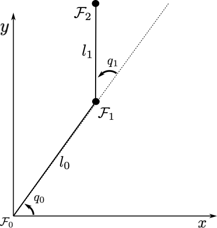
For the 2-DoF planar robot shown in the figure, let $q_0\triangleq q_0(t)$ , $q_1\triangleq q_1(t)$ , $l_{0}$ , $l_{1} \in \mathbb{R}$ be the parameters to calculate

\mymatrix{H}^{0}_{2}( q_0, l_{0},q_1,l_{1}) \in SE(2),

(1)

that is, the forward kinematics model of the 2 DoF planar manipulator with configuration space given by

\myvec{q} = \left[\begin{array}{ccc} q_0 \\ q_1 \end{array}\right].

(2)

and given the analytical Jacobian below

\dot{\myvec{x}}=\mymatrix{J} \dot{\myvec{q}}

(3)

where

\myvec{x} = \left[\begin{array}{ccc} p_{x} \\ p_{y} \\ \phi_{z} \end{array}\right],

(4)

in which $p_{x}$ , $p_{y}$ , and $\phi_{z}$ are, respectively, the $x$ -axis position, the $y$ -axis position, and the $z$ -axis angle of $\mathcal{F}_{2}$ . Notice that $\dot{l}_{0}=\dot{l}_{1}=0$ .

Consider the forward kinematics model calculated as in the past lesson¶

\mymatrix{H}^{0}_{2} = \left[\begin{array}{ccc} \cos{(q_0 + q_1)} & -\sin{(q_0 + q_1)} & l_{0}\cos{q_0} + l_{1}\cos{(q_0 + q_1)}\\ \sin{(q_0 + q_1)} & \cos{(q_0 + q_1)} & l_{0}\sin{q_0} + l_{1}\sin{(q_0 + q_1)}\\ 0 & 0 & 1 \end{array}\right].

(5)

This means that, from inspection,

\begin{align} p_{x} & = l_{0}\cos{q_0} + l_{1}\cos{(q_0 + q_1)} \\ p_{y} & = l_{0}\sin{q_0} + l_{1}\sin{(q_0 + q_1)} \\ \phi_{z} & = q_0 + q_1. \end{align}

(6)

With those, we can obtain the task space values with a function called planar_robot_fkm so that it can be easily reused

def planar_robot_fkm(q):
    """
    q: The configuration space values in radians.
    returns the x, this, the current task space value where x = [p_x p_y phi_z]^T.
    """
    l_0 = 0.2 # The robot parameters. They don't change in time, so they are constant here.
    l_1 = 0.1

    q_0 = q[0] # Just to make it more readable.
    q_1 = q[1] 

    p_x = l_0 * cos(q_0) + l_1 * cos(q_0 + q_1)
    p_y = l_0 * sin(q_0) + l_1 * sin(q_0 + q_1)
    phi_z = q_0 + q_1

    return np.array([p_x,
                     p_y,
                     phi_z])

Consider the analytical Jacobian¶

We first calculate the Jacobian by hand, because programatically there’s nothing for you to do yet. As we did in the previous tutorial, here is the Jacobian

\mymatrix{J} = \left[\begin{array}{ccc} -l_{0}\sin{q_0} - l_{1}\sin{(q_0 + q_1)} & -l_{1}\sin{(q_0 + q_1)} \\ l_{0}\cos{q_0} + l_{1}\cos{(q_0 + q_1)} & l_{1}\cos{(q_0 + q_1)} \\ 1 & 1 \end{array}\right].

(7)

We transform this Jacobian calculation into the function planar_robot_jacobian shown below

def planar_robot_jacobian(q): 
    """
    q: The configuration space values in radians.
    returns the 3x2 Jacobian mapping [q_0 q_1]^T to [px py phi_z]^T.
    """
    l_0 = 0.2 # The robot parameters. They don't change in time, so they are constant here.
    l_1 = 0.1

    q_0 = q[0] # Just to make it more readable.
    q_1 = q[1] 

    J_1_1 = -l_0 * sin(q_0) - l_1 * sin(q_0 + q_1)
    J_1_2 = -l_1 * sin(q_0  + q_1)
    J_2_1 =  l_0 * cos(q_0) + l_1 * cos(q_0 + q_1)
    J_2_2 =  l_1 * cos(q_0 +  q_1)
    J_3_1 = 1
    J_3_2 = 1

    return np.array(
                [[J_1_1, J_1_2],
                 [J_2_1, J_2_2],
                 [J_3_1, J_3_2]]
        )

Kinematic Control¶

1. Define an error function¶

We usually use

\tilde{\myvec{x}}= \myvec{x} - \myvec{x}_d

(8)

that can be implemented as the function get_error below

def get_error(x, xd):
    """In this case, we use the difference as the error.
    x: current task-space vector.
    xd: desired task-space vector.
    """
    return x - xd

2. Define the control loop¶

We resort to the following control law

\myvec{u} = -\eta \mymatrix{J}^{+}\tilde{\myvec{x}}

(9)

that can be easily implemented. Notice that we can resort to np.linalg.pinv() to perform the pseudo inversion. According to its documentation, it implements the Moore-Penrose pseudo-inversion based on the Singular Value Decomposition of all “large” singular values.

For the control loop itself, we use all previous functions. The idea here is to show that the norm of the error decreases with the control action. The desired task space vector will not always be achievable. Nonetheless, we can show, as below, that the control action reduces the task-space error, $\tilde{\myvec{x}}$ .

Let $\eta=0.5$ be the controller gain, $T=0.001$ be the sampling time, and $\myvec{x}_d=\left[\begin{array}{ccc} 0.1 & 0.1 & \frac{\pi}{10} \end{array}\right]^T$ . In addition, let the manipulator start at $t=0$ with $q_0=q_1=0$ .

eta = 0.5 # Controller proportional gain
T = 0.001 # Sampling time
# Define initial values for the joint positions
q_0 = 0.0
q_1 = 0.0
q = np.array([q_0,
              q_1])

# A desired task-space value, defined by the problem at hand
xd = np.array([0.1,
               0.1,
               pi/10])
print(f"xd = {xd}")

# Define a stop criteria, in this case let's control for 10 seconds
t = 0 # Current time

# Lists to store the value of each control iteration
x_tilde_norm_list = []
t_list = []

while t < 10:
    # Calculate task-space value, x
    x = planar_robot_fkm(q)
    # Calculate task-space error, x_tilde
    x_tilde = get_error(x, xd)
    # Get the Jacobian
    J = planar_robot_jacobian(q)
    # Invert the Jacobian, for example, with numpy's implementation of it
    J_inv = np.linalg.pinv(J)
    # Calculate the control action
    u = -eta * J_inv @ x_tilde
    
    ## Store values in the list so that we can print them later
    x_tilde_norm_list.append(np.linalg.norm(x_tilde))
    t_list.append(t)

    ## Variable updated for the next loop
    q = q + u * T # Update law using the sampling time
    t = t + T

xd = [0.1        0.1        0.31415927]

Optional: Print the data¶

To help visualise the behavior of the controller, you can optionally plot the data. These data show that with the defined parameters the qualitative behavior is very close to exponential decay.

However the error does not converge to zero, meaning that the manipulator did not reach its target. Indeed, this is usually the case when the target is outside the reach of the manipulator or all task-space desired values cannot be simultenously satisfied.

plt.plot(t_list,x_tilde_norm_list)
plt.title('(RR) Error exponential decay visualization (Moore-Penrose)')
plt.xlabel("Time [s]")
plt.ylabel("$||\\tilde{ \\bf{x} } (t) ||$")
plt.show()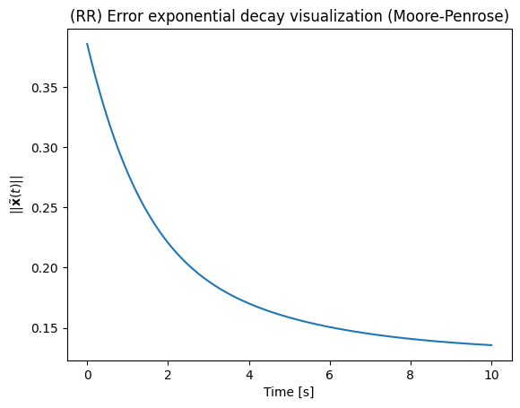

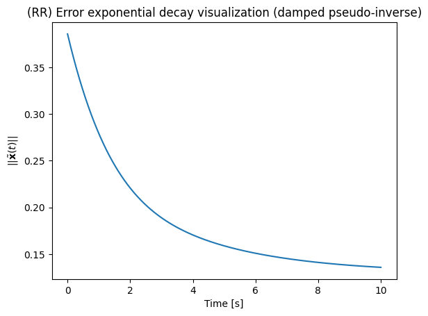
Alternative Jacobian Inversion Strategies¶

The SVD-based Moore-Penrose pseudo-invese is a common strategy for matrix inversion. It is important to notice, however, that is is not the only one. In addition, it is not always the best choice for robot control.

Another common strategy is the so-called damped pseudo-inverse, described below. It is usually the easiest choice to embbed robustness to singularities in the controller.

\mymatrix{J}^{\dagger}=\mymatrix{J}^T\left(\mymatrix{J}\mymatrix{J}^T + \lambda^2\mymatrix{I}\right)^{-1},

(10)

defined in the function damped_pseudo_inverse() below in which we call λ as the variable damping

def damped_pseudo_inverse(A: np.array, damping: float = 0.01):
    """Calculates the damped pseudo inverse of A"""
    if damping == 0:
        raise Exception(f"Damping is {damping} but should be different from zero")
    
    return A.T @ np.linalg.inv(A @ A.T + (damping ** 2) * np.eye(A.shape[0]))

with that, our controller becomes, changing only the inversion strategy,

eta = 0.5 # Controller proportional gain
T = 0.001 # Sampling time
# Define initial values for the joint positions
q_0 = 0.0
q_1 = 0.0
q = np.array([q_0,
              q_1])

# A desired task-space value, defined by the problem at hand
xd = np.array([0.1,
               0.1,
               pi/10])
print(f"xd = {xd}")

# Define a stop criteria, in this case let's control for 10 seconds
t = 0 # Current time

# Lists to store the value of each control iteration
x_tilde_norm_list = []
t_list = []

while t < 10:
    # Calculate task-space value, x
    x = planar_robot_fkm(q)
    # Calculate task-space error, x_tilde
    x_tilde = get_error(x, xd)
    # Get the Jacobian
    J = planar_robot_jacobian(q)
    # Invert the Jacobian using the damped pseudo-inverse
    J_inv = damped_pseudo_inverse(J)
    # Calculate the control action
    u = -eta * J_inv @ x_tilde
    
    ## Store values in the list so that we can print them later
    x_tilde_norm_list.append(np.linalg.norm(x_tilde))
    t_list.append(t)

    ## Variable updated for the next loop
    q = q + u * T # Update law using the sampling time
    t = t + T    

# (Optional) plot the data
plt.plot(t_list,x_tilde_norm_list)
plt.title('(RR) Error exponential decay visualization (damped pseudo-inverse)')
plt.xlabel("Time [s]")
plt.ylabel("$||\\tilde{ \\bf{x} } (t) ||$")
plt.show()

xd = [0.1        0.1        0.31415927]

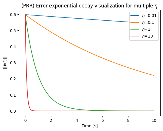
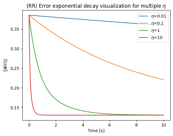
Convergence rate of discrete-time systems¶

Although we usually attempt to find $\myvec{u}$ such that, the error $\tilde{\myvec{x}}$ converges exponentially. This means that, in the right conditions, we will have a convergence

\tilde{\myvec{x}}(t)=\tilde{\myvec{x}}(0)e^{-\eta t}

(11)

in continuous time, hence the convergence depends only on η.

However, given that our implementation is in discrete time, the convergence is affected by our sampling time, $T$ . In practice, we set $T$ as the fastest sampling time that can be achieved by the hardware, e.g. the robot controller. In many cases, this is about 1 milisecond in pratice.

The effect on the convergence for different η can be seen, computationally, below

etas = [0.01, 0.1, 1, 10] # Different gains to iterate over the same control goals
T = 0.001 # Sampling time
# A desired task-space value, defined by the problem at hand
xd = np.array([0.1,
               0.1,
               pi/10])
print(f"xd = {xd}")

# Lists to store the value of each control iteration
x_tilde_norm_list = []
t_list = []
u_norm_list = []

# Run the controller again for each gain
for i in range(0, len(etas)):
    # Define a stop criteria, in this case let's control for 10 seconds
    t = 0 # Current time
    eta = etas[i]
    # Define initial values for the joint positions
    q_0 = 0.0
    q_1 = 0.0
    q = np.array([q_0,
                q_1])
    
    x_tilde_norm_list.append([])
    t_list.append([])
    u_norm_list.append([])

    while t < 10:
        # Calculate task-space value, x
        x = planar_robot_fkm(q)
        # Calculate task-space error, x_tilde
        x_tilde = get_error(x, xd)
        # Get the Jacobian
        J = planar_robot_jacobian(q)
        # Invert the Jacobian using the damped pseudo-inverse
        J_inv = damped_pseudo_inverse(J)
        # Calculate the control action
        u = -eta * J_inv @ x_tilde
        
        ## Store values in the list so that we can print them later
        x_tilde_norm_list[i].append(np.linalg.norm(x_tilde))
        t_list[i].append(t)
        u_norm_list[i].append(np.linalg.norm(u))

        ## Variable updated for the next loop
        q = q + u * T # Update law using the sampling time
        t = t + T    


    plt.plot(t_list[i],x_tilde_norm_list[i], label=f"$\\eta$={eta}")

plt.title('(RR) Error exponential decay visualization for multiple $\\eta$')
plt.legend(loc="upper right")
plt.xlabel("Time [s]")
plt.ylabel("$||\\tilde{ \\bf{x} } (t) ||$")
plt.show()

xd = [0.1        0.1        0.31415927]

Alright, then why don’t we just choose the largest $\eta \approx \infty$ ?¶

Engineering is the art of trade-off. Whenever we have a large η, that means the configuration-space velocities will comparatively be higher.

Using our example, we can see that the control signal norm is heavily affected by η. Therefore, for feasibility, it is important to keep the η so that the system can handle it. In fact, gains that are too high are one of the major risks that can break robots or hurt people when real hardware is used without the proper safeguards.

# Run the controller again for each gain
for i in range(0, len(etas)):
    eta=etas[i]
    plt.plot(t_list[i],u_norm_list[i], label=f"$\\eta$={eta}")

plt.title('(RR) Control signal norm for different $\\eta$')
plt.legend(loc="upper right")
plt.xlabel("Time [s]")
plt.ylabel("$||u (t) ||$")
plt.show()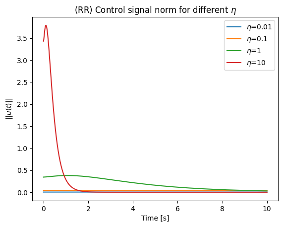

3 DoF Planar Robot (PRR)¶

As you noticed from the previous discussion, what is important for any new robot after you understand these concepts are

Defining a task space, $\myvec{x}$ , that correctly represents the task (and manipulator if applicable).
Obtaining the Forward Kinematics Model (FKM) $f(\myvec{q})=\myvec{x}$ that maps the configuration space, $\myvec{q}$ , to the task space.
Obtaining the analytical Jacobian so that the kinematic control can be applied.
The kinematic control itself, aside from dimensions, does not need to change in general.

For instance, we can even solve with no diagram as long as this information is given. Consider an PRR manipulator with configuration space

\mathbb{R}^3 \ni \myvec{q}_C \triangleq \left[\begin{array}{ccc} q_0 \\ q_1 \\ q_2 \end{array}\right].

(12)

And link lenghts $l_{0}, l_{1}, l_{2}\in \mathbb{R}$ .

Task Space & Forward Kinematics Model (FKM)¶

Let

\begin{align*} s_1 & \triangleq \sin{q_1} \\ s_{12} & \triangleq \sin{(q_1 + q_2)} \\ c_1 & \triangleq \cos{q_1} \\ c_{12} & \triangleq \cos{(q_1 + q_2)}. \end{align*}

(13)

The forward kinematics of this manipulator is therefore given by

SE(2) \ni \mymatrix{H}^{0}_{3}(q_0,q_1,q_2) = \left[\begin{array}{ccc} c_{12} & -s_{12} & (l_0 + q_0) + l_{1}c_{1} + l_{2}c_{12}\\ s_{12} & c_{12} & l_{1}s_{1} + l_{2}s_{12}\\ 0 & 0 & 1 \end{array}\right].

(14)

Because this robot is planar, the following task space is necessary and sufficient to fully describe the reacheable space

\myvec{x} = \left[\begin{array}{ccc} p_{x} \\ p_{y} \\ \phi_{z} \end{array}\right].

(15)

The values can be obtained from inspection of $\mymatrix{H}^{0}_{3}(q_0,q_1,q_2)$ ,

\begin{align*} p_{x} & = (l_0 + q_0) + l_{1}c_{1} + l_{2}c_{12} \\ p_{y} & = l_{1}s_{1} + l_{2}s_{12} \\ \phi_{z} & = q_1 + q_2, \end{align*}

(16)

which means that the FKM, $\myvec{x}=f(\myvec{q})$ , in this case is equivalent to

def planar_robot_prr_fkm(q: np.array) -> np.array:
    """
    q: The configuration space values in radians.
    returns the x, this, the current task space value where x = [p_x p_y phi_z]^T.
    """
    l_0 = 0.2 # The robot parameters. They don't change in time, so they are constant here.
    l_1 = 0.1
    l_2 = 0.3

    q_0 = q[0] # Just to make it more readable.
    q_1 = q[1] 
    q_2 = q[2] 

    s1 = sin(q_1)
    c1 = cos(q_1)
    s12 = sin(q_1 + q_2)
    c12 = cos(q_1 + q_2)

    p_x = (l_0 + q_0) + l_1*c1 + l_2*c12
    p_y = l_1*s1 + l_2*s12
    phi_z = q_1 + q_2

    return np.array([p_x,
                     p_y,
                     phi_z])

Analytical Jacobian¶

The analytical Jacobian is

\mymatrix{J}_C(q_0,q_1,q_2) = \left[\begin{array}{ccc} 1 & - l_{1}s_{1} - l_{2}s_{12} & -l_{2}s_{12}\\ 0 & l_{1}c_{1} + l_{2}c_{12} & l_{2}c_{12}\\ 0 & 1 & 1 \end{array}\right].

(17)

def planar_robot_prr_jacobian(q): 
    """
    q: The configuration space values in radians.
    returns the 3x3 Jacobian mapping [q_0 q_1 q_2]^T to [px py phi_z]^T.
    """
    l_0 = 0.2 # The robot parameters. They don't change in time, so they are constant here.
    l_1 = 0.1
    l_2 = 0.3

    q_0 = q[0] # Just to make it more readable.
    q_1 = q[1] 
    q_2 = q[2] 

    s1 = sin(q_1)
    c1 = cos(q_1)
    s12 = sin(q_1 + q_2)
    c12 = cos(q_1 + q_2)

    J_1_1 = 1
    J_2_1 = 0
    J_3_1 = 0

    J_1_2 = -l_1*s1 - l_2*s12
    J_2_2 = l_1*c1 + l_2*c12
    J_3_2 = 1

    J_1_3 = -l_2*s12
    J_2_3 = l_2*c12
    J_3_3 = 1

    return np.array(
                [[J_1_1, J_1_2, J_1_3],
                 [J_2_1, J_2_2, J_2_3],
                 [J_3_1, J_3_2, J_3_3]]
        )

Kinematic Control¶

With this, a similar control as before, but changing the FKM and Jacobian can be easily achieved. We change only

The configuration space in lines 20 to 25.
planar_robot_prr_fkm in line 33
planar_robot_prr_jacobian in line 37.

The rest of the control loop is unchanged! This is one of the advantages of kinematic control.

etas = [0.01, 0.1, 1, 10] # Different gains to iterate over the same control goals
T = 0.001 # Sampling time
# A desired task-space value, defined by the problem at hand
xd = np.array([0.1,
               0.1,
               pi/10])
print(f"xd = {xd}")

# Lists to store the value of each control iteration
x_tilde_norm_list = []
t_list = []
u_norm_list = []

# Run the controller again for each gain
for i in range(0, len(etas)):
    # Define a stop criteria, in this case let's control for 10 seconds
    t = 0 # Current time
    eta = etas[i]
    # Define initial values for the joint positions
    q_0 = 0.0
    q_1 = 0.0
    q_2 = 0.0
    q = np.array([q_0,
                  q_1,
                  q_2])
    
    x_tilde_norm_list.append([])
    t_list.append([])
    u_norm_list.append([])

    while t < 10:
        # Calculate task-space value, x
        x = planar_robot_prr_fkm(q)
        # Calculate task-space error, x_tilde
        x_tilde = get_error(x, xd)
        # Get the Jacobian
        J = planar_robot_prr_jacobian(q)
        # Invert the Jacobian using the damped pseudo-inverse
        J_inv = damped_pseudo_inverse(J)
        # Calculate the control action
        u = -eta * J_inv @ x_tilde
        
        ## Store values in the list so that we can print them later
        x_tilde_norm_list[i].append(np.linalg.norm(x_tilde))
        t_list[i].append(t)
        u_norm_list[i].append(np.linalg.norm(u))

        ## Variable updated for the next loop
        q = q + u * T # Update law using the sampling time
        t = t + T    


    plt.plot(t_list[i],x_tilde_norm_list[i], label=f"$\\eta$={eta}")

plt.title('(PRR) Error exponential decay visualization for multiple $\\eta$')
plt.legend(loc="upper right")
plt.xlabel("Time [s]")
plt.ylabel("$||\\tilde{ \\bf{x} } (t) ||$")
plt.show()

xd = [0.1        0.1        0.31415927]

Pre-requisites for the learner¶

I found an issue¶

Latex Macros¶

Package installation¶

Imports¶

Suggested exercises¶

2 DoF planar robot (RR)¶

Consider the forward kinematics model calculated as in the past lesson¶

Consider the analytical Jacobian¶

Kinematic Control¶

1. Define an error function¶

2. Define the control loop¶

Optional: Print the data¶

Alternative Jacobian Inversion Strategies¶

Convergence rate of discrete-time systems¶

Alright, then why don’t we just choose the largest η≈∞\eta \approx \inftyη≈∞?¶

3 DoF Planar Robot (PRR)¶

Task Space & Forward Kinematics Model (FKM)¶

Analytical Jacobian¶

Kinematic Control¶

Alright, then why don’t we just choose the largest $\eta \approx \infty$ ?¶