%%capture
'''
(C) Copyright 2020-2025 Murilo Marques Marinho (murilomarinho@ieee.org)

     This file is licensed in the terms of the
     Attribution-NonCommercial-ShareAlike 4.0 International (CC BY-NC-SA 4.0)
     license.

 Derivative work of:
 https://github.com/dqrobotics/learning-dqrobotics-in-matlab/tree/master/robotic_manipulators
 Contributors to this file:
     Murilo Marques Marinho (murilomarinho@ieee.org)
'''

DQ2 Quaternion Basics using DQ Robotics¶

I found an issue¶

Thank you! Please report it at https://github.com/MarinhoLab/OpenExecutableBooksRobotics/issues

Introduction¶

Before going into the topic of quaternions, it is important to review some high-school level math. And, of course, we need to install the library! This is easy to do. The library is available in PyPI.

%%capture
%pip install dqrobotics dqrobotics-pyplot
%pip install dqrobotics dqrobotics-pyplot --break-system-packages

from dqrobotics_extensions.pyplot import plot
import matplotlib.pyplot as plt
from math import pi, cos, sin

Quick review on complex numbers¶

The set of complex numbers $\mathbb{C}$ , can be understood as an extention of the set of real numbers $\mathbb{R}$ . Any complex number can always be written in the form

\mathit{\mathbf{c}}=a+b\hat{\;\imath \;,}

(1)

where $a,b\in \;$ $\mathbb{R}$ . In addition, the imaginary unit, $\hat{\;\imath \;}$ has the following property

{\hat{\;\imath \;} }^2 =-1\ldotp

(2)

For instance, the complex number

{\mathit{\mathbf{c}}}_1 =5+28\hat{\imath \;} \;

(3)

can be written using DQ Robotics as follows.

# Import essential DQ algebra
from dqrobotics import *

# Define c1
c1 = 5 + 28*i_
print(f"c1 = {c1}")

c1 = 5 + 28i

Notice that the imaginary unit property holds:

# Imaginary unit property
i_ * i_

- 1

Note: Do not confuse Python’s “j” with DQ Robotics “j_”. They are different.

import numpy as np

if j_ != 1j:
    print("DQ Robotics j_ is not equal to Python's j")

DQ Robotics j_ is not equal to Python's j

Operations on complex numbers¶

The operations on complex numbers are very similar to the operations on real numbers. We just need to respect the property ${\hat{\;\imath \;} }^2 =-1\ldotp$

For instance, for the complex numbers

c_1 =a_1 +b_1 \hat{\imath \;},

(4)

c_2 =a_2 +b_2 \hat{\imath \;}.

(5)

c1 = 5  + 28*i_
print(f"c1 = {c1}")

c1 = 5 + 28i

c2 = 25 + 88*i_
print(f"c2 = {c2}")

c2 = 25 + 88i

Sum/Subtraction¶

c_3 =c_1 +c_2 =\left(a_1 +a_2 \right)+\left(b_1 +b_2 \right)\hat{\;\imath \;} \ldotp

(6)

c3 = c1 + c2
print(f"c3 = {c3}")

c3 = 30 + 116i

The subtraction is defined accordingly.

{\;c}_1 -c_2 =\left(a_1 -a_2 \right)+\left(b_1 -b_2 \right)\hat{\;\imath \;} \ldotp

(7)

c1 - c2

- 20 - 60i

Product¶

The product will be

{\;c}_1 c_2 =\left(a_1 a_2 -b_1 b_2 \right)+\left(a_1 b_2 +b_1 a_2 \right)\hat{\;\imath \;}.

(8)

c1 * c2

- 2339 + 1140i

Conjugation¶

The conjugate of a complex number is defined as

{\left(c_1 \right)}^* =a-b\hat{\;\imath \;}.

(9)

conj(c1)

5 - 28i

Norm¶

The norm of a complex number can be obtained as

\left|\right|c_1 \left|\right|=\sqrt{c_1 c_1^* \;}=\sqrt{\left(a_1 +b_1 \hat{\imath \;} \right)\left(a_1 -b_1 \hat{\imath \;} \right)\;}=\sqrt{a_1^2 +b_1^2 }.

(10)

norm(c1)

28.442925

Imaginary part¶

The imaginary part is

\textrm{Im}\left(c_1 \right)=b\hat{\;\imath \;}.

(11)

Im(c1)

28i

Real¶

The real part is

\textrm{Re}\left(c_1 \right)=a.

(12)

Re(c1)

5

Quaternions¶

When we extend the concept of complex numbers to four dimensions, we have what we call quaternions. They compose the set $\mathbb{H}$ and can always be written in the form

\mathit{\mathbf{h}}=a+b\hat{\;\imath \;} +c\hat{\;\jmath \;} +d\hat{\;k},

(13)

where $a,b,c,d\in \;$ $\mathbb{R}$ . In addition, the imaginary units $\hat{\;\imath \;}$ , $\hat{\;\jmath \;}$ , and $\hat{\;k\;}$ have the following properties

{\hat{\;\imath \;} }^2 ={\hat{\;\jmath \;} }^2 ={\hat{\;k} }^2 =\hat{\;\imath \;} \hat{\;\jmath \;} \hat{\;k} =-1.

(14)

Note that every complex number is a quaternion, but not every quaternion is a complex number ( $\mathbb{C}\subset \mathbb{H}$ ).

For instance, the quaternion

{\mathit{\mathbf{c}}}_1 =5+28\hat{\imath \;} +85\hat{\;\jmath \;} +99\hat{\;k}

(15)

can be written using DQ Robotics as follows

# Define c1
c1 = 5 + 28*i_ + 86*j_ + 99*k_
print(f"c1 = {c1}")

c1 = 5 + 28i + 86j + 99k

We can verify the properties of the imaginary units in DQ Robotics as follows

i_ * i_

- 1

j_ * j_

- 1

k_ * k_

- 1

i_ * j_ * k_

- 1

Operations on quaternions¶

Considering ${\mathit{\mathbf{h}}}_1 ,{\mathit{\mathbf{h}}}_2 \in \;$ $\mathbb{H}$ , for example

h1 = 5 + 28*i_ + 86*j_ + 99*k_
print(f"h1 = {h1}")

h1 = 5 + 28i + 86j + 99k

h2 = -2 + 25*k_
print(f"h2 = {h1}")

h2 = 5 + 28i + 86j + 99k

Sum/Subtraction¶

{\mathit{\mathbf{h}}}_1 \pm {\mathit{\mathbf{h}}}_2 =\left(a_1 \pm a_2 \right)+\left(b_1 \pm b_2 \right)\hat{\;\imath \;} +\left(c_1 \pm c_2 \right)\hat{\;\jmath \;} +\left(d_1 \pm d_2 \right)\hat{\;k\;}.

(16)

h1 + h2

3 + 28i + 86j + 124k

h1 - h2

7 + 28i + 86j + 74k

Multiplication¶

{\mathit{\mathbf{h}}}_1 {\mathit{\mathbf{h}}}_2 =\textrm{See}\;\textrm{Bonus}\;\textrm{Homework}\;1\ldotp

(17)

h1 * h2

- 2485 + 2094i - 872j - 73k

Notice that the multiplication between quaternions is, in general, NOT COMMUTATIVE.

{\mathit{\mathbf{h}}}_1 {\mathit{\mathbf{h}}}_2 \not= {{\mathit{\mathbf{h}}}_2 \mathit{\mathbf{h}}}_1.

(18)

h3 = h1 * h2

h4 = h2 * h1

if h3==h4:
    print('h1*h2 is equal to h2*h1')
else:
    print('h1*h2 is not equal to h2*h1')

h1*h2 is not equal to h2*h1

It can be commutative in some cases. For instance, consider the trivial case in which $h_1 =h_2$ .

Real part¶

\textrm{Re}\left({\mathit{\mathbf{h}}}_1 \right)=a.

(19)

Re(h1)

5

If the real part of a quaternion is zero, it is called a pure quaternion, and belongs to the set ${\mathbb{H}}_p$ .

Imaginary part¶

\textrm{Im}\left({\mathit{\mathbf{h}}}_1 \right)=b\hat{\;\imath \;} +c\hat{\;\jmath \;} +d\hat{\;k}.

(20)

Im(h1)

28i + 86j + 99k

Conjugation¶

{\left({\mathit{\mathbf{h}}}_1 \right)}^* =\textrm{Re}\left({\mathit{\mathbf{h}}}_1 \right)-\textrm{Im}\left({\mathit{\mathbf{h}}}_1 \right)=a-b\hat{\;\imath \;} -c\hat{\;\jmath \;} -d\hat{\;k}.

(21)

conj(h1)

5 - 28i - 86j - 99k

Norm

\left|\right|{\mathit{\mathbf{h}}}_1 \left|\right|=\sqrt{{\mathit{\mathbf{h}}}_1 {\mathit{\mathbf{h}}}_1^* \;}=\textrm{See}\;\textrm{Bonus}\;\textrm{Homework}\;2\ldotp

(22)

norm(h1)

134.186437

Vec3¶

The imaginary part of the quaternion can be mapped to ${\mathbb{R}}^3$ as follows

{\textrm{vec}}_3 \left({\mathit{\mathbf{h}}}_1 \right)=\left\lbrack \begin{array}{c} b\\ c\\ d \end{array}\right\rbrack.

(23)

vec3(h1)

array([28., 86., 99.])

Vec4¶

Quaternions can be mapped to ${\mathbb{R}}^4$ as follows

{\textrm{vec}}_4 \left({\mathit{\mathbf{h}}}_1 \right)=\left\lbrack \begin{array}{c} a\\ b\\ c\\ d \end{array}\right\rbrack.

(24)

vec4(h1)

array([ 5., 28., 86., 99.])

Hamilton Operators¶

The hamilton operators are useful to provide a form of commutativity in the quaternion multiplication.

{\textrm{vec}}_4 \left({\mathit{\mathbf{h}}}_1 {\mathit{\mathbf{h}}}_2 \right)=\overset{+}{{\mathit{\mathbf{H}}}_4 } \left({\mathit{\mathbf{h}}}_1 \right){\textrm{vec}}_4 \left({\mathit{\mathbf{h}}}_2 \right)=\overset{-}{{\mathit{\mathbf{H}}}_4 } \left({\mathit{\mathbf{h}}}_2 \right){\textrm{vec}}_4 \left({\mathit{\mathbf{h}}}_1 \right).

(25)

vec4(h1*h2)

array([-2485., 2094., -872., -73.])

hamiplus4(h1)*vec4(h2)

array([[  -10.,    -0.,    -0., -2475.],
       [  -56.,     0.,    -0.,  2150.],
       [ -172.,     0.,     0.,  -700.],
       [ -198.,    -0.,     0.,   125.]])

haminus4(h2)*vec4(h1)

array([[  -10.,    -0.,    -0., -2475.],
       [    0.,   -56.,  2150.,    -0.],
       [    0.,  -700.,  -172.,     0.],
       [  125.,     0.,    -0.,  -198.]])

Conjugate mapping matrix¶

The following matrix is useful when the quaternion conjugate is used. For quaternions it is defined as,

{\mathit{\mathbf{C}}}_4 =\left\lbrack \begin{array}{cccc} 1 & 0 & 0 & 0\\ 0 & -1 & 0 & 0\\ 0 & 0 & -1 & 0\\ 0 & 0 & 0 & -1 \end{array}\right\rbrack

(26)

and has the following property

{\mathit{\mathbf{C}}}_4 {\textrm{vec}}_4 \left({\mathit{\mathbf{h}}}_1 \right)={\textrm{vec}}_4 \left({\mathit{\mathbf{h}}}_1^* \right)\ldotp

(27)

Unit quaternions and the rotation of rigid bodies¶

Unit quaternions compose the set ${\mathbb{S}}^3$ , which represent rotations of the reference frame of rigid bodies in three-dimensional space. A unit quaternion can always be written in the form

\mathit{\mathbf{r}}=\cos \left(\frac{\phi }{2}\right)+\textrm{vsin}\left(\frac{\;\phi \;}{2}\right)\left(\textrm{See}\;\textrm{Bonus}\;\textrm{Homework}\;3\right),

(28)

where $\phi \in$ $\mathbb{R}$ is the rotation angle around the rotation axis $v\in$ ${\mathbb{S}}^3 \cap {\mathbb{H}}_p$ (Remember that ${\mathbb{H}}_p$ are pure quaternions, that is, quaternions for which the real part is zero).

Unit-norm quaternions, as the name says, have unit norm

\left|\right|r\left|\right|=1\ldotp

(29)

For instance, to represent the rotation of $\frac{\pi }{2}$ rad about the x-axis, the following quaternion can be used

r_1 =\cos \left(\frac{\;\pi \;}{4}\right)+\hat{\;\imath \;} \sin \left(\frac{\;\pi \;}{4}\right).

(30)

r1 = cos(pi/4) + i_*sin(pi/4)

We can check that $r_1$ indeed has unit norm

norm(r1)

1

Unit quaternion double-cover property¶

Note that the same rotation can be represented by two different quaternions, because

{\mathit{\mathbf{r}}}_1

(31)

and

-{\mathit{\mathbf{r}}}_1

(32)

represent the same resulting rotation but are different quaternions. For instance, see that even though the following two quaternions represent the same rotation.

r1 = 1
print(f"r1 = {r1}")

r1 = 1

r2 = cos(pi) + i_*sin(pi)
print(f"r2 = {r2}")

r2 =  - 1

they have opposite signs.

This is called the “double-cover” property. We will not address this now, but it is important to know that this property exists.

No rotation¶

The quaternion that represents that there is no rotation is

r_1 = 1.

(33)

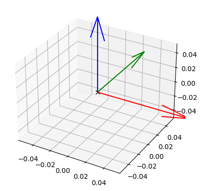
r1 = DQ([1])

Plotting quaternions¶

Using DQ Robotics, the rotation quaternions can be plotted on screen. See, for example

Note: for the unit quaternion $r_1 =1$ , you have to explicitly initialize it using the DQ constructor before plotting, otherwise MATLAB will not use the correct plot function.

print(f'Printing 1 as a quaternion: {r1}')
plt.figure()
ax = plt.axes(projection='3d')
plot(r1)
plt.show()

Printing 1 as a quaternion: 1

Sequential rotations¶

Sequential rotations are obtained by post-multiplication. For example, the transformation between the neutral reference frame by ${r_1 }$ followed by ${r_2 }$ is

{\mathit{\mathbf{r}}}_3 ={\mathit{\mathbf{r}}}_1 {\mathit{\mathbf{r}}}_2.

(34)

For example

from math import pi, cos, sin

r1 = cos(pi/16) + i_*sin(pi/16)
r2 = cos(pi/4) + i_*sin(pi/4)
r3 = r1*r2

plt.figure()
ax = plt.axes(projection='3d')
plot(r3)
plt.show()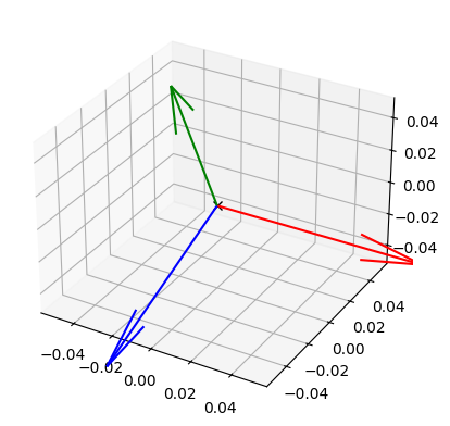

We can also plot all intermediary rotations using subplot.

from math import pi, cos, sin

r1 = cos(pi/16) + i_*sin(pi/16)
r2 = cos(pi/32) + i_*sin(pi/32)
r3 = r1*r2

plt.figure(figsize=(15,5))
ax1 = plt.subplot(1,3,1, projection='3d')
plot(r1)
ax1.title.set_text('r1')
ax2 = plt.subplot(1,3,2, projection='3d')
plot(r2)
ax2.title.set_text('r2')
ax3 = plt.subplot(1,3,3, projection='3d')
plot(r3)
ax3.title.set_text('Rotation of r1 by r2')
plt.show()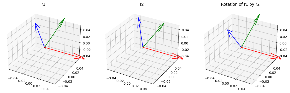

Reverse rotation¶

The reverse rotation can be obtained using the conjugate operation, because unit quaternions have unit norm. Hence,

\mathit{\mathbf{r}}{\left(\mathit{\mathbf{r}}\right)}^* = 1.

(35)

For example, for a given rotation quaternion

r1 = cos(pi/16) + i_*sin(pi/16)

The rotation quaternion that corresponds to the reverse rotation is given by its conjugate.

conj(r1)

0.980785 - 0.19509i

We can verify that sequentially multiplying one by the other gives us a “no rotation” quaternion.

r1 * conj(r1)

1

Homework¶

in the beginning of your script.

Create a MATLAB script called [quaternion_basics_homework.m]. On it, do the following tasks.
Store, in $r_1$ , the value of a rotation of $\phi =\frac{\pi \;\;}{8}\;\textrm{rad}$ about the x-axis.
Store, in $r_2$ , the value of a rotation of $\phi =\frac{\pi \;\;}{16}\;\textrm{rad}$ about the y-axis.
Store, in $r_3$ , the value of a rotation of $\phi =\frac{\pi \;\;}{32}\;\textrm{rad}$ about the z-axis.
Calculate the result of the sequential rotation of the neutral reference-frame by $r_1$ , followed by $r_2$ , followed by $r_3$ , and store it in ${\mathit{\mathbf{r}}}_4$ . Plot ${\mathit{\mathbf{r}}}_4$ .
Find the reverse rotation of ${\mathit{\mathbf{r}}}_4$ and store it in ${\mathit{\mathbf{r}}}_5$ .
Rotate ${\mathit{\mathbf{r}}}_5$ by ${360}^{\circ \;}$ about the x-axis and store it in ${\mathit{\mathbf{r}}}_6$ . Is ${\mathit{\mathbf{r}}}_5 =-{\mathit{\mathbf{r}}}_6$ ? Plot ${\mathit{\mathbf{r}}}_5$ and ${\mathit{\mathbf{r}}}_6$ to confirm that they represent the same rotation.

Bonus Homework¶

What is the general form of the quaternion multiplication? Multiply ${\mathit{\mathbf{h}}}_1 =a_1 +b_1 \hat{\;\imath \;} +c_1 \hat{\;\jmath \;} +d_1 \hat{\;k}$ and ${\mathit{\mathbf{h}}}_2 =a_2 +b_2 \hat{\;\imath \;} +c_2 \hat{\;\jmath \;} +d_2 \hat{\;k}$ on pen and paper and find ${\mathit{\mathbf{h}}}_3 =a_3 +b_3 \hat{\;\imath \;} +c_3 \hat{\;\jmath \;} +d_3 \hat{\;k}$ .
What is the general form of the quaternion norm? Simplify $\sqrt{\;{\mathit{\mathbf{h}}}_1 {\mathit{\mathbf{h}}}_1^* }$ on pen and paper.
Show that every unit quaternion, written as $\mathit{\mathbf{r}}=\cos \left(\frac{\phi }{2}\right)+\textrm{vsin}\left(\frac{\;\phi \;}{2}\right)$ , has unit norm. Do that on pen and paper.