DQ5 Robot Control Basics using DQ Robotics - Part 1¶

I found an issue¶

Thank you! Please report it at https://github.com/MarinhoLab/OpenExecutableBooksRobotics/issues

$\providecommand{\myvec}[1]{{\mathbf{\boldsymbol{{#1}}}}}$ $\providecommand{\mymatrix}[1]{{\mathbf{\boldsymbol{{#1}}}}}$ $\providecommand{\quat}[1]{{\mathbf{\boldsymbol{{#1}}}}}$ $\providecommand{\dual}{\varepsilon}$

Introduction¶

For now, we have studied how dual quaternions can be a powerful algebraic tool to represent interesting geometric elements, such as reference frames, planes, lines, and points.

In this lesson we will study the control of very basic robots.

As always, before we start, make essential installations and imports.

Notation¶

Keep these in mind (we will also use this notation when writting papers to conferences and journals):

• $h\in \mathbb{H}$ : a quaternion. (Bold-face, lowercase character)
• $\underline{h} \in \mathcal{H}$ : a dual quaternion. (Bold-face, underlined, lowercase character)
• $p,t,\cdots \in {\mathbb{H}}_p$ : pure quaternions. They represent points, positions, and translations. They are quaternions for which $\textrm{Re}\left(h\right)=0$ .
• $r\in {\mathbb{S}}^3$ : unit quaternions. They represent orientations and rotations. They are quaternions for which $||h||=1$ .
• $\underline{x} \in$ $\underline{\mathcal{S}}$ : unit dual quaternions. They represent poses and pose transformations. They are dual quaternions for which $||h||=1$ .
• $\underline{l} \in {\mathcal{H}}_p \cap$ $\underline{{\mathcal{S}}}$ : a Plücker line.
• $\underline{{{\pi }}} \in \left\lbrace P\left(\underline{{{\pi }}} \right)\in {\mathbb{H}}_p \right\rbrace \cap \underline{{\mathcal{S}}}$ : a plane.

Basics of Robot Kinematic Control¶

At this point, most robotics textbooks will introduce you to the kinematic modeling of robotic manipulators in detail.

Let us start with a one degree-of-freedom (DoF) planar robot, so that we can understand some major points regarding robotic control before we start making more complicated robotic modeling.

1-DoF planar robot¶

We start by defining the important reference frames, the robot, and the task we want to accomplish. We call this, “Problem Definition”.

Problem Definition¶

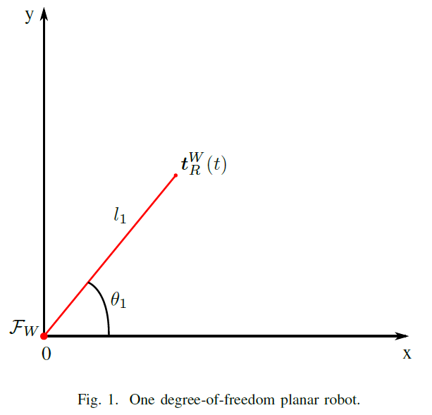
1. Let the robot $R$ be a 1-DoF planar robot, as drawn in Fig.1.
2. Let ${\mathcal{F}}_W$ be the world-reference frame.
3. Let ${\underline{x} }_R^W (t)$ $\in$ $\underline{\mathcal{S}}$ represent the time-dependent transformation from the origin of the world-reference frame to the tip of the robot. The tip of the robot is called end effector. Note that ${\underline{x} }_R^W (t)$ has a superscript “W” that means that the reference frame of this pose transformation is ${\mathcal{F}}_W$ . The subscript “R” means that, after the pose transformation, we will be at the end effector of the robot $R$ .
4. Let $R$ be composed of single link, actuated by a rotational joint that rotates about its z-axis by an angle $\theta_1 (t)\in \mathbb{R}$ . The reference frame of the joint coincides with ${\mathcal{F}}_W$ when $\theta_1 (t)=0$ . The length of the link is $l_1 \in$ ${\mathbb{R}}^+ -\lbrace 0\rbrace$ .
5. Consider that we can freely control the variable $\theta_1 (t)\triangleq \theta_1$ . The robot is said to have one degree-of-freedom because it has only one independent joint value.

Problems:

1. Obtain the forward kinematic model and the inverse kinematic model of the robot $R$ that maps the joint value, $\theta_1 (t)$ , to the 3D translation of the end effector, $t_R^W (t)\triangleq \textrm{translation}\left({\underline{x} }_R^W \right)$ using unit dual quaternions. This can be easily found using simple trigonometry, but we will slowly move to more complicated examples.
2. Obtain the differential kinematic model and the inverse differential kinematic model of the robot $R$ .
3. Using 1. and 2., design an open-loop velocity controller in task-space.
4. Using 1. and 2., design a closed-loop position controller in task-space.

Forward Kinematic Model¶

The forward kinematic model (FKM), concerns finding the function that maps the joint space variables into the task space variables.

• The joint space variables are all joint variables that we can control. In the current example, the joint space is only $\theta_1 (t)$ .
• The task space variables depend on the task, but in general are the pose, the translation, the rotation, etc of the end effector. In the current example, the task space is the end-effector’s translation $t_R^W (t)$ .
• The FKM answers the question: what is the end-effector {pose, translation, rotation, etc}, given its joint values?

Note the kinematic model of a robot models the motion of the robot without considering forces. It concerns only the geometry of the robot. This means that weight, inertia, and so on are not considered in kinematic modeling.

The FKM of robot $R$ is quite straigthforward, and can be found using two pose transformations.

where

is the rotation about the joint value (remember that the rotational joint pivots about its z-axis) and

is the translation of $l_1$ about the rotated x-axis.

DQ Robotics Example¶

Let us create a class representing the 1-DoF planar robot. To keep our code organized, we write it in a separate file in snake case [one_dof_planar_robot.py]. The length of the robot does not change in time, so we add it as a class property.

Let us follow the Google Python Style Guide as much as possible, so that your code is readable.

1. Class names should be written in camel-case, starting with an uppercase letter. For example “OneDofPlanarRobot”.
2. Properties and methods should be written in lowercase, possibly using “_” if needed. For instance, “l”, or “fkm()” or “my_favorite_method()”
3. Add comments to help other people understand what you are doing.

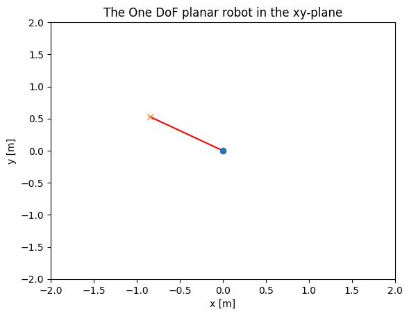
Inverse Kinematic Model¶

In most robotic control tasks, the task is defined in terms of the task-space variables, such as $t_R^W (t)$ , and not in terms of the joint-space variables, such as $\theta_1 (t)$ . For instance, “move the end effector to a given position”.

The inverse kinematic model (IKM), concerns finding the opposite mapping of the FKM, that is, a function that maps the task space variables into joint space variables.

• The FKM answers the question: what is the joint value I need so that the robot’s end effector goes to a desired {pose, translation, rotation, etc}?

We can start from the FKM

note that the total pose transformation is

By the definition of the translation operation for any $\underline{x}$ $\in$ $\underline{\mathcal{S}}$

Using the operation above and two trigonometric identities, we reach the following

This form is quite straightforward for us to find the IKM. Given that we the robot has only one degree-of-freedom, in this situation we can either choose to control the x-axis translation OR the y-axis translation. The other is defined by our initial choise.

For simplicity, let us define

where $t_x ,t_y ,t_z \in$ $\mathbb{R}$ represent the 3D coordinates of the robot’s end effector.

Moreover, notice that, even in this very simple case, we have an issue. There are two possible values for $\theta_1$ that give us the same $t_x$ , and the same for $t_y$ . When finding an IKM, we have to simply choose one of the possible cases. We will adress alternative solutions afterwards, so in practice we almost never have to find the IKM explicitly.

If we decide to choose the x-axis translation, we have

And if we decide to choose the y-axis translation, we have

Note that, for all cases,

When the robot does not have enough degrees-of-freedom for a specific task, we call it underactuated. In this case, the planar robot does not have enough degrees-of-freedom for us to freely choose the x-axis and y-axis translation simultaneously.

DQ Robotics Example¶

The following methods are relevant

Suppose that $t_x$ is to be controlled.

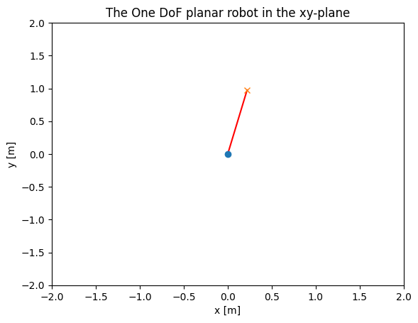
Now, suppose that $t_y$ is to be controlled.

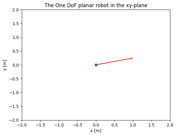
Differential Kinematics Model¶

The first-order time-derivative of the FKM is called Differential Kinematics Model (DKM). It maps the joint-space velocities into task-space velocities. Although maybe not obvious at first glance, inverting the DKM is considerably easier than finding the IK high-DoF robots.

Back to our example, the DKM of the 1-DoF planar robot is the first-order time-derivative of the FKM

Notice that it does not depend on the time-derivative of $l_1$ because $l_1$ does not vary on time (in this example). Let us call

then, our DKM becomes,

We can write this in matrix form as

In this case, the matrix

is, in general, called task Jacobian. Given that this specific Jacobian is related to the translation, we call it translation Jacobian. Note that the translation Jacobian depends on the joint value.

DQ Robotics Example¶

We add the following method to our 1-DoF planar robot.

Inverse Differential Kinematics Model¶

The inverse differential kinematics model (IDKM) is the inverse relation of the DKM: it maps task-space velocities into joint-space velocities.

By inspecting our DKM, see how easy it is to invert the relation. We just need to left-multiply the equation by some type of inverse of the translation Jacobian. For instance, we can choose

which results in

In practice, instead of finding a pseudo-inverse algebraically, we use numerical methods to find the (pseudo) inverse of the task Jacobian.

Note: You certainly learned already that the inverse of a matrix only exists when the matrix is square and full-rank. For all other cases, you can resort to pseudo-inverses.

DQ Robotics Example¶

Using dqrobotics.utils.DQ_LinearAlgebra, we have an implementation of the singular-value decomposition pseudo-inverse to calculate the IDKM called pinv.

Task-space Velocity Control using the IDKM¶

We are now equipped to design a simple open-loop task-space velocity controller.

In our example with the 1-DoF planar robot, let the goal be to have the a constant task-space velocity, ${\dot{t} }_d \in {\mathbb{H}}_p$ .

Given the open-loop design, we can directly plug in the desired task-space velocity in the IDKM, which results in

Some robots will allow you to control the joint velocity directly. However, for some robots you will only be able to control the joint positions. In this case, you can discretize the controller as follows

where $\tau \in {\mathbb{R}}^+ -\lbrace 0\rbrace$ is the sampling time.

DQ Robotics Example¶

For the following example, the discretized version of the open-loop velocity controller was implemented. You can change vx, vy, and vz.

We can plot the results of the simulations using the following function, which was implemented in plot_td_dot_and_t_dot.py

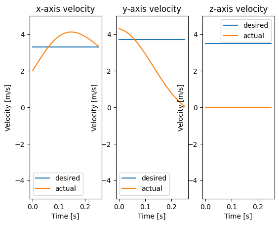
Note that, in general, this simple robot cannot mantain the desired velocity. The main reason for this is the geometry of the 1-DoF planar robot. As shown in detail when the IK was calculated, the velocity in the x-axis and the y-axis are coupled. In addition, we cannot control the velocity in the z-axis.

Task-space position control using the IDKM¶

Controlling the task-space variables (translation, rotation, or pose) directly is in general more useful than controlling their velocities.

In our example with the 1-DoF planar robot, let the goal be to reach a given task-space translation, $\quat{t}_d \in {\mathbb{H}}_p$ .

To do so, we start with the IDKM

Remember that we can freely choose a ${\dot{\quat{t}} }_R^W (t)$ that is relevant to our task. Let us choose

with $\eta \in {\mathbb{R}}^+ -\lbrace 0\rbrace$ . The parameter η is used to control the convergence speed.

The position controller becomes

for $\tilde{t} =\left(t_R^W -{{t_d}}\right)$ .

Note that $\tilde{t}$ is a vector that points from the current end-effector position to the desired end-effector position. It is a type of error function.

Error convergence¶

When designing controllers, it is important to guarantee that error norm converges to zero when time tends to infinity. In our example, this means

When can show that this is true by inspecting the error dynamics under certain assumptions. We do that by getting the first-order time-derivative of the error function. In our example,

because the desired translation does not vary on time. Then, we can substitute the DKM to find

then, we can replace our controller

in general, we suppose that

where $\mymatrix{I}$ is the identity matrix of suitable size. Hence, we have that

Which means that the error exponentially converges to zero when time tends to infinity.

Note: In fact, the equation $\mymatrix {J}_t \mymatrix{J}_t^{\textrm{inv}} = \mymatrix{I}$ does not hold in many situations (it also doesn’t hold in our example, because of the coupling between the translations in the x-axis and the y-axis, and the z-axis translation can’t be controlled at all). The point of this section is not to discuss this in detail, but just to give the reader a general idea of the reasoning behind task-space position control.

DQ Robotics Example¶

Homework¶

(1) Following the format of [OneDofPlanarRobot.m], create a class called [TwoDofPlanarRobot.m] that represents a 2-DoF planar robot as shown in the following figure $l_1 ,l_2 \in {\mathbb{R}}^+ -0$ and $\theta_1 ,\theta_2 \in \mathbb{R}$ .

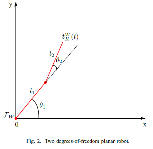
The class must have

1. A constructor that takes $l_1 ,l_2$ as inputs.
2. A function that calculates the forward kinematics model (FKM) of the robot.
3. A function that calculates the translation Jacobian of the robot.
4. A plot function that plots the robot in 2D space.

Note: You do NOT need to implement the IK function.

(2) With the class you created in (1), create a script called two_dof_planar_robot_position_control.py that implements a task-space translation controller. Control the robot from the initial posture $\theta_1 (0)=0,\theta_2 (0)=\frac{\pi }{2}$ to $t_d =2\hat{\jmath}$ .